$ \def\D{\mathcal{D}} \def\ipar{m} \def\R{\mathbb{R}} \def\del{\partial} \def\vec{\bf} \def\priorm{\mu_0} \def\C{\mathcal{C}} \def\Acal{\mathcal{A}} \def\postm{\mu_{\rm{post}}} \def\iparpost{\ipar_\text{post}} \def\obs{\vec{d}} \def\yobs{\obs^{\text{obs}}} \def\obsop{\mathcal{B}} \def\dd{\vec{\bar{d}}} \def\iFF{\mathcal{F}} \def\iFFadj{\mathcal{F}^*} \def\ncov{\Gamma_{\mathrm{noise}}} $
Example: Bayesian initial condition inversion in an advection-diffusion problem
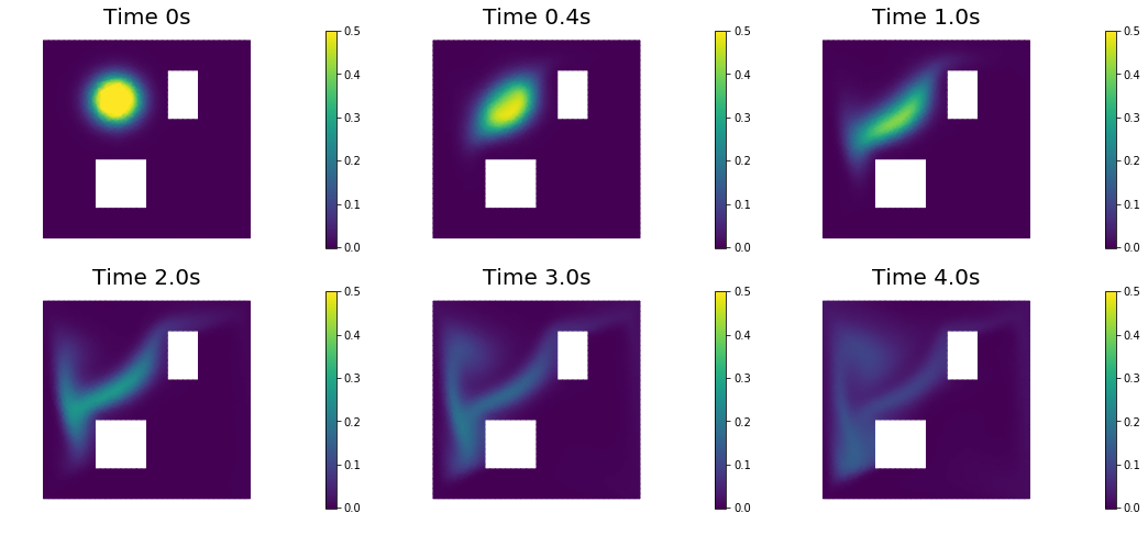
In this example we tackle the problem of quantifying the uncertainty in the solution of an inverse problem governed by a parabolic PDE via the Bayesian inference framework. The underlying PDE is a time-dependent advection-diffusion equation in which we seek to infer an unknown initial condition from spatio-temporal point measurements.
The Bayesian inverse problem:
Following the Bayesian framework, we utilize a Gaussian prior measure $\priorm = \mathcal{N}(\ipar_0,\C_0)$, with $\C_0=\Acal^{-2}$ where $\Acal$ is an elliptic differential operator as described in the PoissonBayesian example, and use an additive Gaussian noise model. Therefore, the solution of the Bayesian inverse problem is the posterior measure, $\postm = \mathcal{N}(\iparpost,\C_\text{post})$ with $\iparpost$ and $\C_\text{post}$.
- The posterior mean $\iparpost$ is characterized as the minimizer of
which can also be interpreted as the regularized functional to be minimized in deterministic inversion. The observation operator $\mathcal{B}$ extracts the values of the forward solution $u$ on a set of locations ${\vec{x}_1, \ldots, \vec{x}_n} \subset \D$ at times ${t_1, \ldots, t_N} \subset [0, T]$.
- The posterior covariance $\C_{\text{post}}$ is the inverse of the Hessian of $\mathcal{J}(\ipar)$, i.e.,
The forward problem:
The PDE in the parameter-to-observable map $\iFF$ models diffusive transport in a domain $\D \subset \R^d$ ($d \in {2, 3}$):
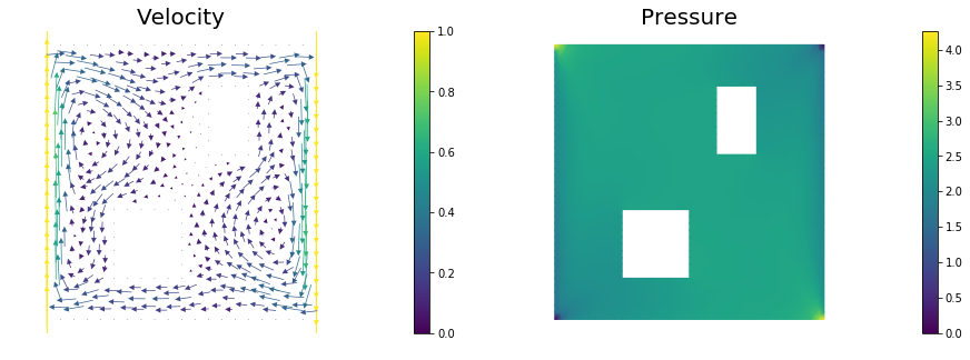
Here, $\kappa > 0$ is the diffusion coefficient and $T > 0$ is the final time. The velocity field $\vec{v}$ is computed by solving the following steady-state Navier-Stokes equation with the side walls driving the flow:
Here, $q$ is pressure, $\text{Re}$ is the Reynolds number. The Dirichlet boundary data $\vec{g} \in \R^d$ is given by $\vec{g} = \vec{e}_2$ on the left wall of the domain, $\vec{g}=-\vec{e}_2$ on the right wall, and $\vec{g} = \vec{0}$ everywhere else.
The adjoint problem:
1. Load modules
from __future__ import absolute_import, division, print_function

import dolfin as dl
import math
import numpy as np
import matplotlib.pyplot as plt
%matplotlib inline
import sys
sys.path.append( "../hippylib" )
from hippylib import *
sys.path.append( "../hippylib/applications/ad_diff/" )
from model_ad_diff import TimeDependentAD
sys.path.append( "../hippylib/tutorial" )
import nb

import logging
logging.getLogger('FFC').setLevel(logging.WARNING)
logging.getLogger('UFL').setLevel(logging.WARNING)
dl.set_log_active(False)

np.random.seed(1)
2. Construct the velocity field
def v_boundary(x,on_boundary):
    return on_boundary

def q_boundary(x,on_boundary):
    return x[0] < dl.DOLFIN_EPS and x[1] < dl.DOLFIN_EPS

def computeVelocityField(mesh):
    Xh = dl.VectorFunctionSpace(mesh,'Lagrange', 2)
    Wh = dl.FunctionSpace(mesh, 'Lagrange', 1)
    if dlversion() <= (1,6,0):
        XW = dl.MixedFunctionSpace([Xh, Wh])
    else:
        mixed_element = dl.MixedElement([Xh.ufl_element(), Wh.ufl_element()])
        XW = dl.FunctionSpace(mesh, mixed_element)

    Re = 1e2

    g = dl.Expression(('0.0','(x[0] < 1e-14) - (x[0] > 1 - 1e-14)'), degree=1)
    bc1 = dl.DirichletBC(XW.sub(0), g, v_boundary)
    bc2 = dl.DirichletBC(XW.sub(1), dl.Constant(0), q_boundary, 'pointwise')
    bcs = [bc1, bc2]

    vq = dl.Function(XW)
    (v,q) = dl.split(vq)
    (v_test, q_test) = dl.TestFunctions (XW)

    def strain(v):
        return dl.sym(dl.nabla_grad(v))

    F = ( (2./Re)*dl.inner(strain(v),strain(v_test))+ dl.inner (dl.nabla_grad(v)*v, v_test)
           - (q * dl.div(v_test)) + ( dl.div(v) * q_test) ) * dl.dx

    dl.solve(F == 0, vq, bcs, solver_parameters={"newton_solver":
                                         {"relative_tolerance":1e-4, "maximum_iterations":100}})

    plt.figure(figsize=(15,5))
    vh = dl.project(v,Xh)
    qh = dl.project(q,Wh)
    nb.plot(nb.coarsen_v(vh), subplot_loc=121,mytitle="Velocity")
    nb.plot(qh, subplot_loc=122,mytitle="Pressure")
    plt.show()

    return v
3. Set up the mesh and finite element spaces
mesh = dl.refine( dl.Mesh("ad_20.xml") )
wind_velocity = computeVelocityField(mesh)
Vh = dl.FunctionSpace(mesh, "Lagrange", 1)
print("Number of dofs: {0}".format( Vh.dim() ) )
Number of dofs: 2023
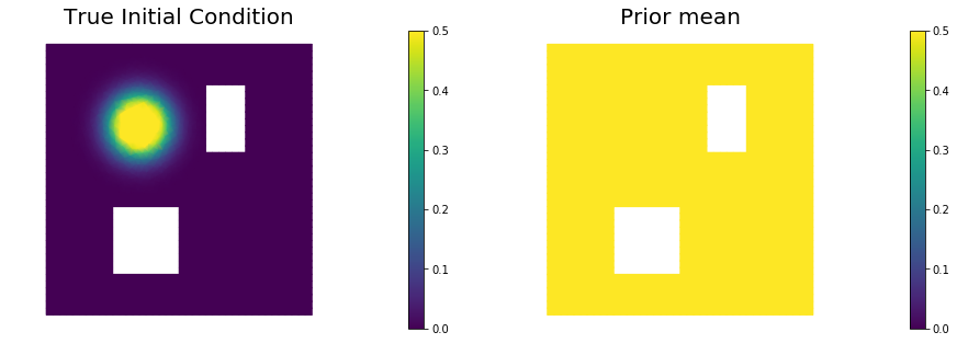
4. Set up model (prior, true/proposed initial condition)
gamma = 1
delta = 8
prior = BiLaplacianPrior(Vh, gamma, delta)

prior.mean = dl.interpolate(dl.Constant(0.5), Vh).vector()
true_initial_condition = dl.interpolate(dl.Expression('min(0.5,exp(-100*(pow(x[0]-0.35,2) +  pow(x[1]-0.7,2))))', degree=5), Vh).vector()
problem = TimeDependentAD(mesh, [Vh,Vh,Vh], 0., 4., 1., .2, wind_velocity, True, prior)

objs = [dl.Function(Vh,true_initial_condition),
        dl.Function(Vh,prior.mean)]
mytitles = ["True Initial Condition", "Prior mean"]
nb.multi1_plot(objs, mytitles)
plt.show()
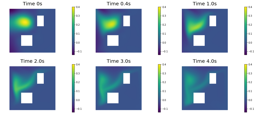
5. Generate the synthetic observations
rel_noise = 0.001
utrue = problem.generate_vector(STATE)
x = [utrue, true_initial_condition, None]
problem.solveFwd(x[STATE], x, 1e-9)
MAX = utrue.norm("linf", "linf")
noise_std_dev = rel_noise * MAX
problem.ud.copy(utrue)
problem.ud.randn_perturb(noise_std_dev)
problem.noise_variance = noise_std_dev*noise_std_dev

nb.show_solution(Vh, true_initial_condition, utrue, "Solution")
6. Test the gradient and the Hessian of the cost (negative log posterior)
m0 = true_initial_condition.copy()
modelVerify(problem, m0, 1e-12, is_quadratic=True)
(yy, H xx) - (xx, H yy) = -4.67531044933e-14

7. Evaluate the gradient
[u,m,p] = problem.generate_vector()
problem.solveFwd(u, [u,m,p], 1e-12)
problem.solveAdj(p, [u,m,p], 1e-12)
mg = problem.generate_vector(PARAMETER)
grad_norm = problem.evalGradientParameter([u,m,p], mg)

print("(g,g) = ", grad_norm)
(g,g) = 1.66716039169e+12
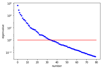
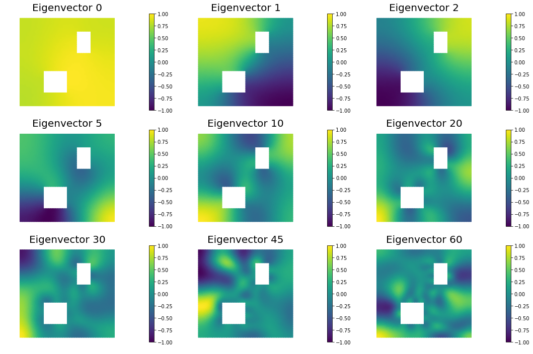
8. The Gaussian approximation of the posterior
H = ReducedHessian(problem, 1e-12, gauss_newton_approx=False, misfit_only=True)

k = 80
p = 20
print("Single Pass Algorithm. Requested eigenvectors: {0}; Oversampling {1}.".format(k,p))
Omega = np.random.randn(m.array().shape[0], k+p)
lmbda, V = singlePassG(H, prior.R, prior.Rsolver, Omega, k)


posterior = GaussianLRPosterior( prior, lmbda, V )

plt.plot(range(0,k), lmbda, 'b*', range(0,k+1), np.ones(k+1), '-r')
plt.yscale('log')
plt.xlabel('number')
plt.ylabel('eigenvalue')

nb.plot_eigenvectors(Vh, V, mytitle="Eigenvector", which=[0,1,2,5,10,20,30,45,60])
Single Pass Algorithm. Requested eigenvectors: 80; Oversampling 20.
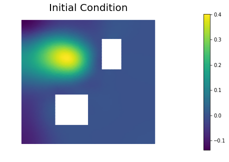
9. Compute the MAP point
H.misfit_only = False

solver = CGSolverSteihaug()
solver.set_operator(H)
solver.set_preconditioner( posterior.Hlr )
solver.parameters["print_level"] = 1
solver.parameters["rel_tolerance"] = 1e-6
solver.solve(m, -mg)
problem.solveFwd(u, [u,m,p], 1e-12)

total_cost, reg_cost, misfit_cost = problem.cost([u,m,p])
print("Total cost {0:5g}; Reg Cost {1:5g}; Misfit {2:5g}".format(total_cost, reg_cost, misfit_cost))

posterior.mean = m

plt.figure(figsize=(7.5,5))
nb.plot(dl.Function(Vh, m), mytitle="Initial Condition")
plt.show()

nb.show_solution(Vh, m, u, "Solution")
 Iterartion :  0  (B r, r) =  30140.7469368
 Iteration :  1  (B r, r) =  0.0653730893942
 Iteration :  2  (B r, r) =  6.28009167641e-06
 Iteration :  3  (B r, r) =  9.57006671181e-10
Relative/Absolute residual less than tol
Converged in  3  iterations with final norm  3.09355244207e-05
Total cost 84.2612; Reg Cost 68.8823; Misfit 15.3789
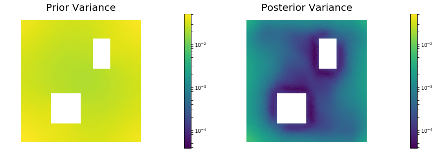
10. Prior and posterior pointwise variance fields
compute_trace = True
if compute_trace:
    post_tr, prior_tr, corr_tr = posterior.trace(method="Estimator", tol=5e-2, min_iter=20, max_iter=2000)
    print("Posterior trace {0:5g}; Prior trace {1:5g}; Correction trace {2:5g}".format(post_tr, prior_tr, corr_tr))
post_pw_variance, pr_pw_variance, corr_pw_variance = posterior.pointwise_variance("Exact")

objs = [dl.Function(Vh, pr_pw_variance),
        dl.Function(Vh, post_pw_variance)]
mytitles = ["Prior Variance", "Posterior Variance"]
nb.multi1_plot(objs, mytitles, logscale=True)
plt.show()
Posterior trace 0.000465642; Prior trace 0.0284301; Correction trace 0.0279644
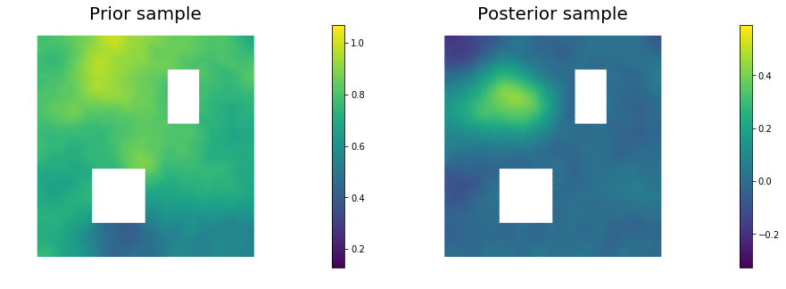
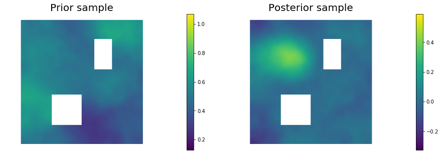
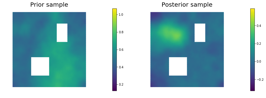
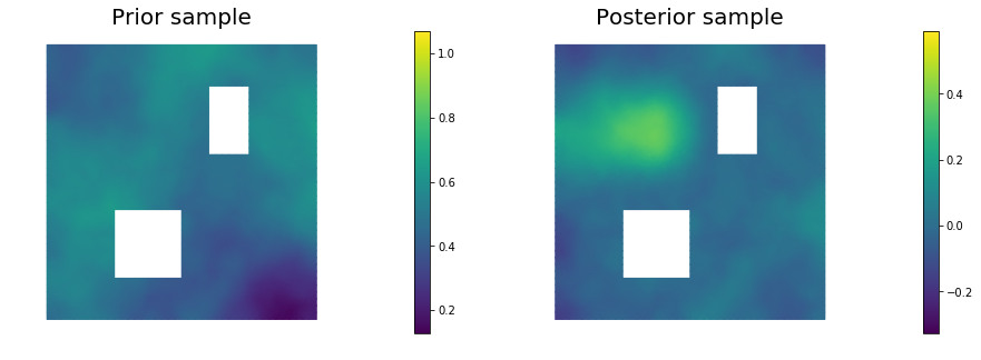
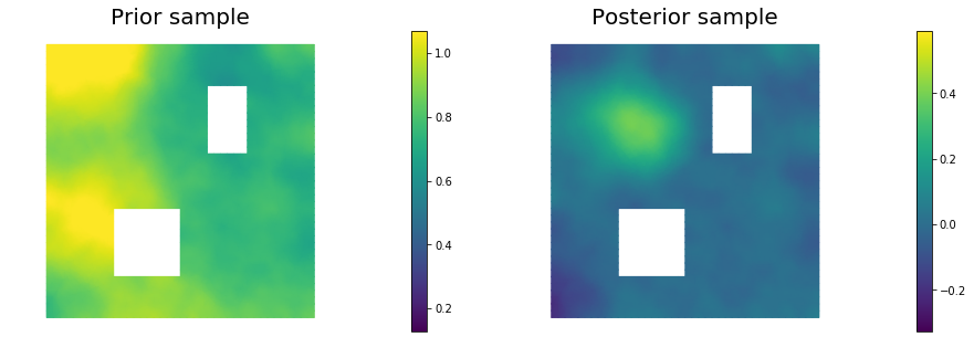
11. Draw samples from the prior and posterior distributions
nsamples = 5
noise = dl.Vector()
posterior.init_vector(noise,"noise")
noise_size = noise.array().shape[0]
s_prior = dl.Function(Vh, name="sample_prior")
s_post = dl.Function(Vh, name="sample_post")

pr_max =  2.5*math.sqrt( pr_pw_variance.max() ) + prior.mean.max()
pr_min = -2.5*math.sqrt( pr_pw_variance.min() ) + prior.mean.min()
ps_max =  2.5*math.sqrt( post_pw_variance.max() ) + posterior.mean.max()
ps_min = -2.5*math.sqrt( post_pw_variance.max() ) + posterior.mean.min()

for i in range(nsamples):
    noise.set_local( np.random.randn( noise_size ) )
    posterior.sample(noise, s_prior.vector(), s_post.vector())
    plt.figure(figsize=(15,5))
    nb.plot(s_prior, subplot_loc=121,mytitle="Prior sample", vmin=pr_min, vmax=pr_max)
    nb.plot(s_post, subplot_loc=122,mytitle="Posterior sample", vmin=ps_min, vmax=ps_max)
    plt.show()
Copyright (c) 2016-2017, The University of Texas at Austin & University of California, Merced. All Rights reserved. See file COPYRIGHT for details.
This file is part of the hIPPYlib library. For more information and source code availability see https://hippylib.github.io.
hIPPYlib is free software; you can redistribute it and/or modify it under the terms of the GNU General Public License (as published by the Free Software Foundation) version 2.0 dated June 1991.