Spectrum of the preconditioned Hessian misfit operator

The linear source inversion problem

We consider the following linear source inversion problem. Find the state $u \in H^1_{\Gamma_D}(\Omega)$ and the source (parameter) $m \in H^1(\Omega)$ that solves

$\begin{aligned} {} & \min_, \frac{1}{2} \| Bu - u_d \|^2 + \frac{1}{2} \int_\Omega \left[ \delta|m-m_0|^2 + \gamma|\nabla (m - m_0)|^2 \right] dx & {}\\ {\rm s.t.} & {} &{} \\ {} & -{\rm div}(k \nabla u) + {\bf v}\cdot \nabla u + cu = m & {\rm in} \; \Omega\\ {} & u = 0 & {\rm on } \; \Gamma_D\\ {} & k \frac{\partial u}{\partial n} = 0 & {\rm on } \; \Gamma_N\\ \end{aligned}$

Here:

$u_d$ is a $n_{\rm obs}$ finite dimensional vector that denotes noisy observations of the state $u$ in $n_{\rm obs}$ locations $\mathbf{x}_i$ , $i=1,\ldots,n_{\rm obs}$ . Specifically, $u_d(i) = u_{\rm true}( {\bf x}_i ) + \eta_i$ , where $\eta_i$ are i.i.d. $\mathcal{N}(0, \sigma^2)$ .
$B: H^1_0(\Omega) \rightarrow {R}^{n_{\rm obs}}$ is the linear operator that evaluates the state $u$ at the observation locations $\mathbf{x}_i$ , $i=1,\ldots,n_{\rm obs}$ .
$\delta$ and $\gamma$ are the parameters of the regularization penalizing the $L^2(\Omega)$ and $H^1(\Omega)$ norm of $m-m_0$, respectively.
$k$, ${\bf v}$, $c$ are given coefficients representing the diffusivity coefficient, the advective velocity and the reaction term, respectively.
$\Gamma_D \subset \partial \Omega$, $\Gamma_N \subset \partial \Omega$ represents the subdomain of $\partial\Omega$ where we impose Dirichlet or Neumann boundary conditions, respectively.

1. Load modules

import matplotlib.pyplot as plt
%matplotlib inline

import dolfin as dl
import numpy as np

import sys
sys.path.append("../hippylib")
from hippylib import *
sys.path.append("../hippylib/tutorial")
import nb

import logging
logging.getLogger('FFC').setLevel(logging.WARNING)
logging.getLogger('UFL').setLevel(logging.WARNING)
dl.set_log_active(False)

/usr/local/lib/python2.7/dist-packages/matplotlib/__init__.py:1401: UserWarning:  This call to matplotlib.use() has no effect
because the backend has already been chosen;
matplotlib.use() must be called *before* pylab, matplotlib.pyplot,
or matplotlib.backends is imported for the first time.

  warnings.warn(_use_error_msg)

2. The linear source inversion problem

def A_varf(u,p):
    return k*dl.inner(dl.nabla_grad(u), dl.nabla_grad(p))*dl.dx \
           + dl.inner(dl.nabla_grad(u), v*p)*dl.dx \
           + c*u*p*dl.dx
        
def f_varf(p):
    return dl.Constant(0.)*p*dl.dx
        
def C_varf(m,p):
           return -m*p*dl.dx
    
def R_varf(m_trial, m_test, gamma, delta):
    return dl.Constant(delta)*m_trial*m_test*dl.dx \
           + dl.Constant(gamma)*dl.inner(dl.grad(m_trial), dl.grad(m_test))*dl.dx

def u_boundary(x, on_boundary):
    return on_boundary and x[1] < dl.DOLFIN_EPS

class Hessian:
    def __init__(self, A_solver,C,B,R):
        self.misfit_only = False
        self.A_solver = A_solver
        self.C = C
        self.B = B
        self.R = R
        
        self.uhat = dl.Vector()
        self.C.init_vector(self.uhat,0)
        self.fwd_rhs = dl.Vector()
        self.C.init_vector(self.fwd_rhs,0)
        self.adj_rhs = dl.Vector()
        self.C.init_vector(self.adj_rhs,0)
        self.phat = dl.Vector()
        self.C.init_vector(self.phat,0)
        
    def init_vector(self, x, dim):
        self.R.init_vector(x,dim)
        
    def mult(self, x, y):
        y.zero()
        self.C.mult(x, self.fwd_rhs)
        self.A_solver.solve(self.uhat, self.fwd_rhs)
        self.B.transpmult(self.B*self.uhat, self.adj_rhs)
        self.A_solver.solve_transpose(self.phat, self.adj_rhs)
        self.C.transpmult(self.phat, y)
        
        if not self.misfit_only:
            y.axpy(1., self.R*x)
        

def solve(nx, ny, targets, gamma, delta, verbose=True):
    np.random.seed(seed=2)
    mesh = dl.UnitSquareMesh(nx, ny)
    Vh1 = dl.FunctionSpace(mesh, 'Lagrange', 1)
    
    Vh = [Vh1, Vh1, Vh1]
    if verbose:
        print "Number of dofs: STATE={0}, PARAMETER={1}, ADJOINT={2}".format(Vh[STATE].dim(), Vh[PARAMETER].dim(), Vh[ADJOINT].dim())


    u_bdr = dl.Constant(0.0)
    bc = dl.DirichletBC(Vh[STATE], u_bdr, u_boundary)
    
    u_trial = dl.TrialFunction(Vh[STATE])
    u_test  = dl.TestFunction(Vh[STATE])
    m_trial = dl.TrialFunction(Vh[PARAMETER])
    m_test  = dl.TestFunction(Vh[PARAMETER])
    
    A,f = dl.assemble_system(A_varf(u_trial, u_test), f_varf(u_test), bcs =bc )
    A_solver = dl.PETScLUSolver()
    A_solver.set_operator(A)
    C = dl.assemble(C_varf(m_trial, u_test))
    bc.zero(C)
    
    R = dl.assemble(R_varf(m_trial, m_test, gamma, delta))
    R_solver = dl.PETScLUSolver()
    R_solver.set_operator(R)

    mtrue = dl.interpolate(
        dl.Expression('min(0.5,exp(-100*(pow(x[0]-0.35,2) +  pow(x[1]-0.7,2))))',degree=5), Vh[PARAMETER]).vector()
    m0 = dl.interpolate(dl.Constant(0.0), Vh[PARAMETER]).vector()
     
    if verbose:
        print "Number of observation points: {0}".format(targets.shape[0])
    
    B = assemblePointwiseObservation(Vh[STATE], targets)
               
    #Generate synthetic observations
    utrue = dl.Function(Vh[STATE]).vector()
    A_solver.solve(utrue, -(C*mtrue) )
    d = B*utrue
    MAX = d.norm("linf")
    rel_noise = 0.01
    noise_std_dev = rel_noise * MAX
    randn_perturb(d, noise_std_dev)

    u = dl.Function(Vh[STATE]).vector()
    m = m0.copy()
    p = dl.Function(Vh[ADJOINT]).vector()
    mg = dl.Function(Vh[PARAMETER]).vector()
    rhs_adj = dl.Function(Vh[STATE]).vector()
    
    # Solve forward:
    A_solver.solve(u, -(C*m) )
    # rhs for adjoint
    B.transpmult(d-(B*u), rhs_adj)
    # solve adj problem
    A_solver.solve_transpose(p, rhs_adj)
    #gradient
    C.transpmult(p, mg)
    mg.axpy(1., R*m)
   

    H = Hessian(A_solver,C,B,R)

    solver = CGSolverSteihaug()
    solver.set_operator(H)
    solver.set_preconditioner( R_solver )
    solver.parameters["print_level"] = -1
    solver.parameters["rel_tolerance"] = 1e-9
    solver.solve(m, -mg)

    if solver.converged:
        if verbose:
            print "CG converged in ", solver.iter, " iterations."
    else:
        print "CG did not converged."
        raise

    # Solve forward:
    A_solver.solve(u, -(C*m) )
 
    if verbose:
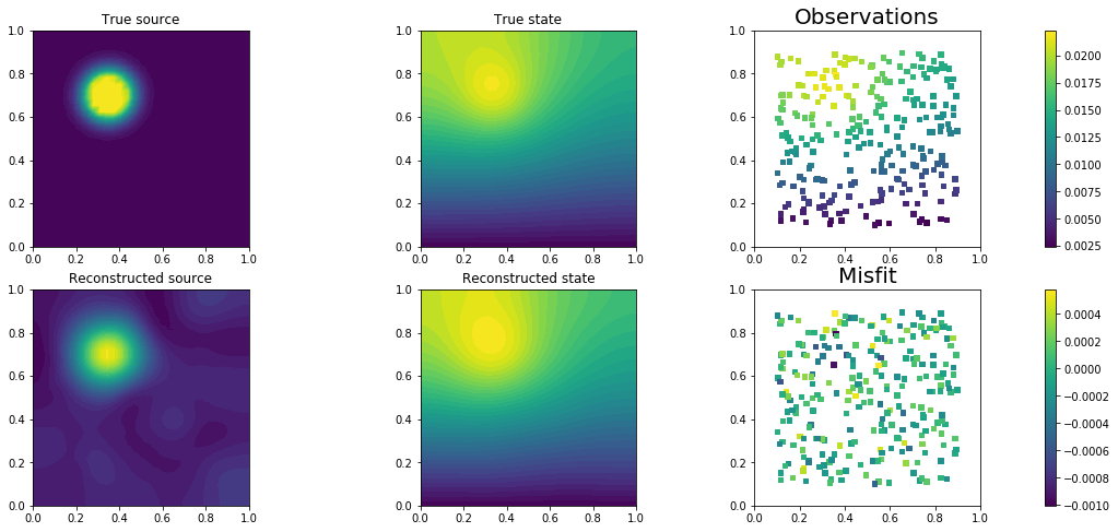
        plt.figure(figsize=(18,8))
        plt.subplot(2, 3, 1)
        dl.plot(dl.Function(Vh[PARAMETER], mtrue), title = "True source")
        plt.subplot(2, 3, 2)
        dl.plot(dl.Function(Vh[STATE], utrue), title="True state")
        plt.subplot(2, 3, 3)
        nb.plot_pts(targets, d,mytitle="Observations")
        plt.subplot(2, 3, 4)
        dl.plot(dl.Function(Vh[PARAMETER], m), title = "Reconstructed source")
        plt.subplot(2, 3, 5)
        dl.plot(dl.Function(Vh[STATE], u), title="Reconstructed state")
        plt.subplot(2, 3, 6)
        nb.plot_pts(targets, B*u-d,mytitle="Misfit")
        plt.show()

    H.misfit_only = True
    k_evec = 80
    p_evec = 5
    if verbose:
        print "Double Pass Algorithm. Requested eigenvectors: {0}; Oversampling {1}.".format(k_evec,p_evec)
    Omega = np.random.randn(m.array().shape[0], k_evec+p_evec)
    lmda, U = doublePassG(H, R, R_solver, Omega, k_evec)

    if verbose:
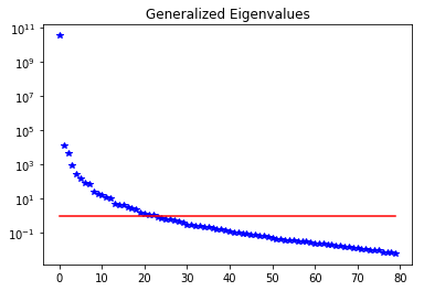
        plt.figure()
        nb.plot_eigenvalues(lmda, mytitle="Generalized Eigenvalues")
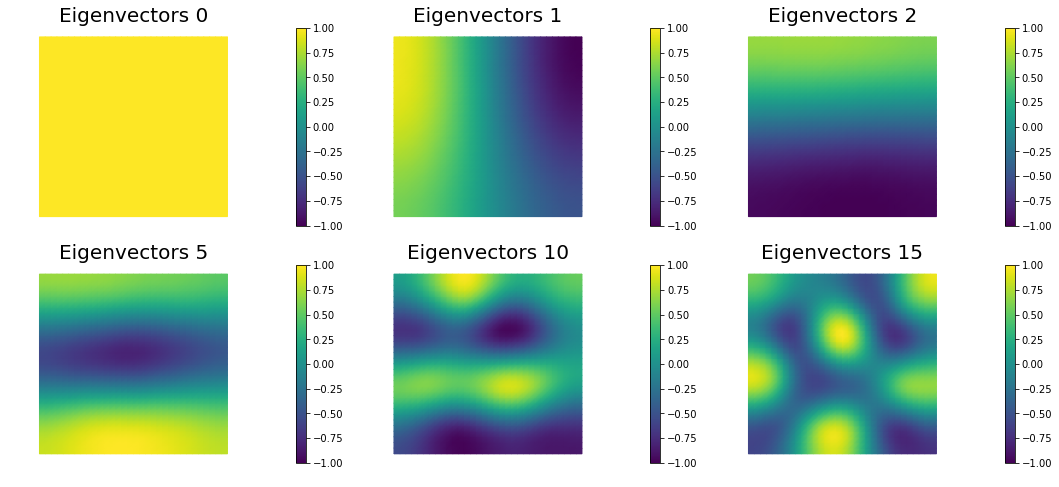
        nb.plot_eigenvectors(Vh[PARAMETER], U, mytitle="Eigenvectors", which=[0,1,2,5,10,15])
        plt.show()
        
    return lmda, U, Vh[PARAMETER], solver.iter

3. Solution of the source inversion problem

ndim = 2
nx = 32
ny = 32

ntargets = 256
np.random.seed(seed=1)
targets = np.random.uniform(0.1,0.9, [ntargets, ndim] )


gamma = 1e-5
delta = 1e-9

k = dl.Constant(1.0)
v = dl.Constant((0.0, 0.0))
c = dl.Constant(0.1)

d, U, Va, nit = solve(nx,ny, targets, gamma, delta)

Number of dofs: STATE=1089, PARAMETER=1089, ADJOINT=1089
Number of observation points: 256
CG converged in  37  iterations.

png

Double Pass Algorithm. Requested eigenvectors: 80; Oversampling 5.

png

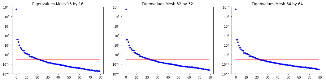
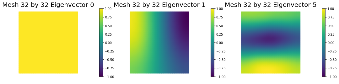
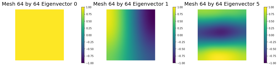
4. Mesh independence of the spectrum of the preconditioned Hessian misfit

gamma = 1e-5
delta = 1e-9

k = dl.Constant(1.0)
v = dl.Constant((0.0, 0.0))
c = dl.Constant(0.1)

n = [16,32,64]
d1, U1, Va1, niter1 = solve(n[0],n[0], targets, gamma, delta,verbose=False)
d2, U2, Va2, niter2 = solve(n[1],n[1], targets, gamma, delta,verbose=False)
d3, U3, Va3, niter3 = solve(n[2],n[2], targets, gamma, delta,verbose=False)

print "Number of Iterations: ", niter1, niter2, niter3
plt.figure(figsize=(18,4))
nb.plot_eigenvalues(d1, mytitle="Eigenvalues Mesh {0} by {1}".format(n[0],n[0]), subplot_loc=131)
plt.ylim([1e-3,1e11])
nb.plot_eigenvalues(d2, mytitle="Eigenvalues Mesh {0} by {1}".format(n[1],n[1]), subplot_loc=132)
plt.ylim([1e-3,1e11])
nb.plot_eigenvalues(d3, mytitle="Eigenvalues Mesh {0} by {1}".format(n[2],n[2]), subplot_loc=133)
plt.ylim([1e-3,1e11])

nb.plot_eigenvectors(Va1, U1, mytitle="Mesh {0} by {1} Eigenvector".format(n[0],n[0]), which=[0,1,5])
nb.plot_eigenvectors(Va2, U2, mytitle="Mesh {0} by {1} Eigenvector".format(n[1],n[1]), which=[0,1,5])
nb.plot_eigenvectors(Va3, U3, mytitle="Mesh {0} by {1} Eigenvector".format(n[2],n[2]), which=[0,1,5])

plt.show()

Number of Iterations:  37 37 37

png

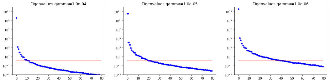
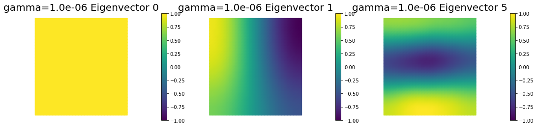
5. Dependence on regularization parameters

We solve the problem for different values of the regularization parameters.

gamma = [1e-4, 1e-5, 1e-6]
delta = [1e-8, 1e-9, 1e-10]

k = dl.Constant(1.0)
v = dl.Constant((0.0, 0.0))
c = dl.Constant(0.1)

d1, U1, Va1, niter1 = solve(nx,ny, targets, gamma[0], delta[0],verbose=False)
d2, U2, Va2, niter2 = solve(nx,ny, targets, gamma[1], delta[1],verbose=False)
d3, U3, Va3, niter3 = solve(nx,ny, targets, gamma[2], delta[2],verbose=False)

print "Number of Iterations: ", niter1, niter2, niter3
plt.figure(figsize=(18,4))
nb.plot_eigenvalues(d1, mytitle="Eigenvalues gamma={0:1.1e}".format(gamma[0]), subplot_loc=131)
plt.ylim([1e-3,1e12])
nb.plot_eigenvalues(d2, mytitle="Eigenvalues gamma={0:1.1e}".format(gamma[1]), subplot_loc=132)
plt.ylim([1e-3,1e12])
nb.plot_eigenvalues(d3, mytitle="Eigenvalues gamma={0:1.1e}".format(gamma[2]), subplot_loc=133)
plt.ylim([1e-3,1e12])

nb.plot_eigenvectors(Va1, U1, mytitle="gamma={0:1.1e} Eigenvector".format(gamma[0]), which=[0,1,5])
nb.plot_eigenvectors(Va2, U2, mytitle="gamma={0:1.1e} Eigenvector".format(gamma[1]), which=[0,1,5])
nb.plot_eigenvectors(Va3, U3, mytitle="gamma={0:1.1e} Eigenvector".format(gamma[2]), which=[0,1,5])

plt.show()

Number of Iterations:  22 37 63

png

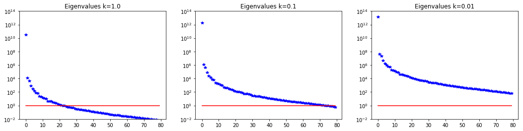
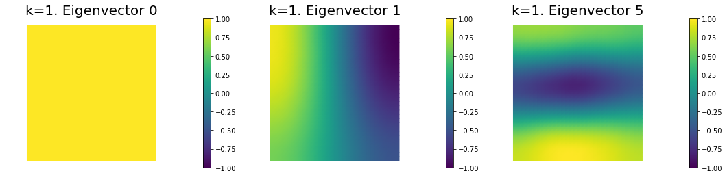
6. Dependence on the PDE coefficients

Assume a constant reaction term $c = 0.1$, and we consider different values for the diffusivity coefficient $k$.

The smaller the value of $k$ the slower the decay in the spectrum.

gamma = 1e-5
delta = 1e-9

k = dl.Constant(1.0)
v = dl.Constant((0.0, 0.0))
c = dl.Constant(0.1)

d1, U1, Va1, niter1 = solve(nx,ny, targets, gamma, delta,verbose=False)
k = dl.Constant(0.1)
d2, U2, Va2, niter2 = solve(nx,ny, targets, gamma, delta,verbose=False)
k = dl.Constant(0.01)
d3, U3, Va3, niter3 = solve(nx,ny, targets, gamma, delta,verbose=False)

print "Number of Iterations: ", niter1, niter2, niter3
plt.figure(figsize=(18,4))
nb.plot_eigenvalues(d1, mytitle="Eigenvalues k=1.0", subplot_loc=131)
plt.ylim([1e-2,1e14])
nb.plot_eigenvalues(d2, mytitle="Eigenvalues k=0.1", subplot_loc=132)
plt.ylim([1e-2,1e14])
nb.plot_eigenvalues(d3, mytitle="Eigenvalues k=0.01", subplot_loc=133)
plt.ylim([1e-2,1e14])

nb.plot_eigenvectors(Va1, U1, mytitle="k=1. Eigenvector", which=[0,1,5])
nb.plot_eigenvectors(Va2, U2, mytitle="k=0.1 Eigenvector", which=[0,1,5])
nb.plot_eigenvectors(Va3, U3, mytitle="k=0.01 Eigenvector", which=[0,1,5])

plt.show()

Number of Iterations:  37 124 746

png

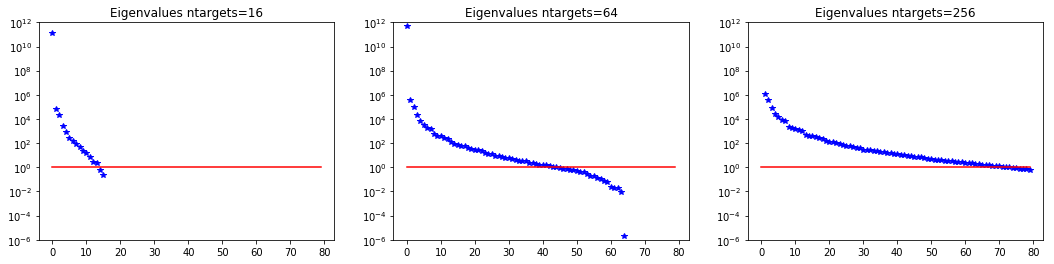
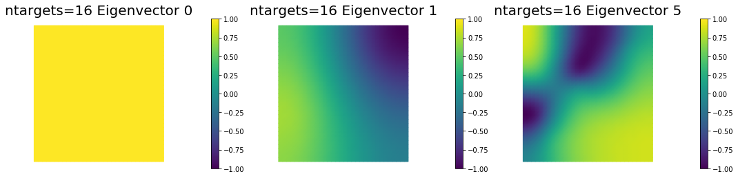
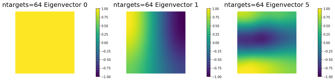
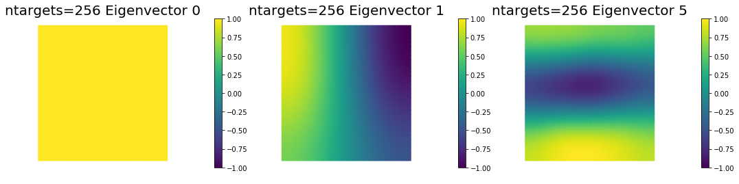
7. Dependence on the number of observations

ntargets = [16, 64, 256]

gamma = 1e-5
delta = 1e-9

k = dl.Constant(0.1)
v = dl.Constant((0.0, 0.0))
c = dl.Constant(0.1)

d1, U1, Va1, niter1 = solve(nx,ny, targets[0:ntargets[0],:], gamma, delta,verbose=False)
d2, U2, Va2, niter2 = solve(nx,ny, targets[0:ntargets[1],:], gamma, delta,verbose=False)
d3, U3, Va3, niter3 = solve(nx,ny, targets[0:ntargets[2],:], gamma, delta,verbose=False)

print "Number of Iterations: ", niter1, niter2, niter3
plt.figure(figsize=(18,4))
nb.plot_eigenvalues(d1, mytitle="Eigenvalues ntargets={0}".format(ntargets[0]), subplot_loc=131)
plt.ylim([1e-6,1e12])
nb.plot_eigenvalues(d2, mytitle="Eigenvalues ntargets={0}".format(ntargets[1]), subplot_loc=132)
plt.ylim([1e-6,1e12])
nb.plot_eigenvalues(d3, mytitle="Eigenvalues ntargets={0}".format(ntargets[2]), subplot_loc=133)
plt.ylim([1e-6,1e12])

nb.plot_eigenvectors(Va1, U1, mytitle="ntargets={0} Eigenvector".format(ntargets[0]), which=[0,1,5])
nb.plot_eigenvectors(Va2, U2, mytitle="ntargets={0} Eigenvector".format(ntargets[1]), which=[0,1,5])
nb.plot_eigenvectors(Va3, U3, mytitle="ntargets={0} Eigenvector".format(ntargets[2]), which=[0,1,5])

plt.show()

Number of Iterations:  31 84 124

png

This file is part of the hIPPYlib library. For more information and source code availability see https://hippylib.github.io.

hIPPYlib is free software; you can redistribute it and/or modify it under the terms of the GNU General Public License (as published by the Free Software Foundation) version 2.0 dated June 1991.

Computational and Variational Methods for Inverse Problems

Fall 2017, CSE 397/GEO 391/ME 397/ORI 397
Prof. O. Ghattas & Dr. U. Villa
Jupyter Notebooks

Spectrum of the preconditioned Hessian misfit operator

The linear source inversion problem

1. Load modules

2. The linear source inversion problem

3. Solution of the source inversion problem

4. Mesh independence of the spectrum of the preconditioned Hessian misfit

5. Dependence on regularization parameters

6. Dependence on the PDE coefficients

7. Dependence on the number of observations

Computational and Variational Methods for Inverse Problems

Fall 2017, CSE 397/GEO 391/ME 397/ORI 397Prof. O. Ghattas & Dr. U. VillaJupyter Notebooks

Spectrum of the preconditioned Hessian misfit operator

The linear source inversion problem

1. Load modules

2. The linear source inversion problem

3. Solution of the source inversion problem

4. Mesh independence of the spectrum of the preconditioned Hessian misfit

5. Dependence on regularization parameters

6. Dependence on the PDE coefficients

7. Dependence on the number of observations

Fall 2017, CSE 397/GEO 391/ME 397/ORI 397
Prof. O. Ghattas & Dr. U. Villa
Jupyter Notebooks