Computational and Variational Methods for Inverse Problems

Poisson Equation in 2D

In this tutorial we solve the Poisson equation in two space dimensions.

For a domain $\Omega \subset \mathbb{R}^2$ with boundary $\partial \Omega = \Gamma_D \cup \Gamma_N$, we write the boundary value problem (BVP):

Here, $\Gamma_D \subset \Omega$ denotes the part of the boundary where we prescribe Dirichlet boundary conditions, and $\Gamma_N \subset \Omega$ denotes the part of the boundary where we prescribe Neumann boundary conditions. $\boldsymbol{n}$ denotes the unit normal of $\partial \Omega$ pointing outside $\Omega$.

To obtain the weak form we define the functional spaces $V_{u_D} := { u \in H^1(\Omega): \, u = u_D \text{ on } \Gamma_D }$ and $V_{0} := { u \in H^1(\Omega): \, u = 0 \text{ on } \Gamma_D }$. Then we multiply the strong form by an arbitrary function $v \in V_0$ and integrate over $\Omega$:

Integration by parts of the non-conforming term gives

Recalling that $v = 0$ on $\Gamma_D$ and that $\nabla u \cdot \boldsymbol{n} = g$ on $\Gamma_N$, the weak form of the BVP is the following.

Find $u \in V_{u_D}$:

To obtain the finite element discretization we then introduce a triangulation (mesh) $\mathcal{T}_h$ of the domain $\Omega$ and we define a finite dimensional subspace $V_h \subset H^1(\Omega)$ consiting of globally continuous functions that are piecewise polynomial on each element of $\mathcal{T}_h$.

The finite element method then reads:

Find $u_h \in V_h$ such that:

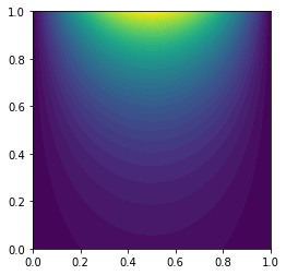
In what follow, we will let $\Omega := [0,1]\times[0,1]$ be the unit square, $\Gamma_N := { (x,y) \in \partial\Omega: y = 1}$ be the top boundary, and $\Gamma_D := \partial\Omega \setminus \Gamma_N$ be the union of the left, bottom, and right boundaries. The coefficient $f$, $g$, $u_D$ are chosen such that the analytical solution is $u_ex = e^{\pi y} \sin(\pi x)$.

1. Imports

We import the following Python packages:

• dolfin is the python interface to FEniCS.
• matplotlib is a plotting library that produces figure similar to the Matlab ones.
• math is the python built-in library of mathematical functions.

# Enable plotting inside the notebook
import matplotlib.pyplot as plt
%matplotlib inline

# Import FEniCS
from dolfin import *
import math

import logging
logging.getLogger('FFC').setLevel(logging.WARNING)
logging.getLogger('UFL').setLevel(logging.WARNING)
set_log_active(False)

2. Define the mesh and the finite element space

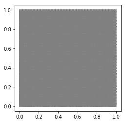
We define a triangulation (mesh) of the unit square $\Omega = [0,1]\times[0,1]$ with n elements in each direction. The mesh size $h$ is $\frac{1}{n}$.

We also define the finite element space $V_h$ as the space of globally continuos functions that are piecewise polinomial (of degree $d$) on the elements of the mesh.

n = 64
d = 1
mesh = UnitSquareMesh(n, n)
Vh = FunctionSpace(mesh, "Lagrange", d)
print "Number of dofs", Vh.dim()
plot(mesh)

Number of dofs 4225

3. Define the Dirichlet boundary condition

We define the Dirichlet boundary condition $u = u_d := \sin(\pi x)$ on $\Gamma_D$.

def boundary_d(x, on_boundary):
    return (x[1] < DOLFIN_EPS or x[0] < DOLFIN_EPS or x[0] > 1.0 - DOLFIN_EPS) and on_boundary

u_d  = Expression("sin(DOLFIN_PI*x[0])", degree = d+2)
bcs = [DirichletBC(Vh, u_d, boundary_d)]

4. Define the variational problem

We write the variational problem $a(u_h, v_h) = F(v_h)$. Here, the bilinear form $a$ and the linear form $L$ are defined as

• $a(u_h, v_h) := \int_\Omega \nabla u_h \cdot \nabla v_h \, dx$
• $L(v_h) := \int_\Omega f v_h \, dx + \int_{\Gamma_N} g \, v_h \, dx$.

$u_h$ denotes the trial function and $v_h$ denotes the test function. The coefficients $f = 0$ and $g = \pi\, e^{\pi y} \sin( \pi x) $ are also given.

uh = TrialFunction(Vh)
vh = TestFunction(Vh)

f = Constant(0.)
g = Expression("DOLFIN_PI*exp(DOLFIN_PI*x[1])*sin(DOLFIN_PI*x[0])", degree=d+2)
a = inner(grad(uh), grad(vh))*dx
L = f*vh*dx + g*vh*ds

5. Assemble and solve the finite element discrete problem

We now assemble the finite element stiffness matrix $A$ and the right hand side vector $b$. Dirichlet boundary conditions are applied at the end of the finite element assembly procedure and before solving the resulting linear system of equations.

A, b = assemble_system(a, L, bcs)
uh = Function(Vh)
solve(A, uh.vector(), b)

plot(uh)

6. Compute error norms

We then compute the $L^2(\Omega)$ and the energy norm of the difference between the exact solution and the finite element approximation.

u_ex = Expression("exp(DOLFIN_PI*x[1])*sin(DOLFIN_PI*x[0])", degree = d+2, domain=mesh)
grad_u_ex = Expression( ("DOLFIN_PI*exp(DOLFIN_PI*x[1])*cos(DOLFIN_PI*x[0])",
                         "DOLFIN_PI*exp(DOLFIN_PI*x[1])*sin(DOLFIN_PI*x[0])"), degree = d+2, domain=mesh )

norm_u_ex   = math.sqrt(assemble(u_ex**2*dx))
norm_grad_ex = math.sqrt(assemble(inner(grad_u_ex, grad_u_ex)*dx))

err_L2   = math.sqrt(assemble((uh - u_ex)**2*dx))
err_grad = math.sqrt(assemble(inner(grad(uh) - grad_u_ex, grad(uh) - grad_u_ex)*dx))

print "|| u_ex - u_h ||_L2 / || u_ex ||_L2 = ", err_L2/norm_u_ex
print "|| grad(u_ex - u_h)||_L2 / = || grad(u_ex)||_L2 ", err_grad/norm_grad_ex

|| u_ex - u_h ||_L2 / || u_ex ||_L2 =  0.000426753981953
|| grad(u_ex - u_h)||_L2 / = || grad(u_ex)||_L2  0.0245370404851