An illustrative example

1D Inverse Heat Equation

An illustrative example is the inversion for the initial condition for a one-dimensional heat equation.

Specifically, we consider a rod of lenght $L$, and we are interested in reconstructing the initial temperature profile $m$ given some noisy measurements $d$ of the temperature profile at a later time $T$.

Forward problem

Given

the initial temperature profile $u(x,0) = m(x)$,
the termal diffusivity $k$,
a prescribed temperature $u(0,t) = u(L,t) = 0$ at the extremities of the rod;

solve the heat equation

$\left\{ \begin{array}{ll} \frac{\partial u}{\partial t} - k \frac{\partial^2}{\partial x^2} u = 0 & \forall x\,\in\,(0, L)\; \forall t \in (0,T)\\ u(x, 0) = m(x) & \forall x \in [0,L] \\ u(0,t) = u(L,t) = 0 & \forall t \in (0, T],\\ \end{array} \right.$

and observe the temperature at the final time $T$:

$\mathcal{F}(m) = u(x, T).$

Analytical solution to the forward problem.

Verify that if

$m(x) = \sin\left(n\, \frac{\pi}{L} x \right), \quad n = 1,2,3, \ldots ,$

then

$u(x,t) = e^{ -k\left(n\, \frac{\pi}{L} \right)^2 t} \sin\left(n\,\frac{\pi}{L} x \right)$

is the unique solution to the heat equation.

Inverse problem

Given the forward model $\mathcal{F}$ and a noisy measurament $d$ of the temperature profile at time $T$, find the initial temperature profile $m$ such that

$\mathcal{F}(m) = d.$

Ill-posedness of the inverse problem

Consider a perturbation

$\delta m(x) = \varepsilon \sin\left(n \, \frac{\pi}{L} x \right),$

where $\varepsilon > 0$ and $n = 1, 2, 3, \ldots$.

Then, by linearity of the forward model $\mathcal{F}$, the corresponding perturbation $\delta d(x) = \mathcal{F}(m + \delta m) - \mathcal{F}(m)$ is

$\delta d(x) = \varepsilon\, e^{ -k\left(n \, \frac{\pi}{L}\right)^2 T} \sin\left(n \, \frac{\pi}{L} x \right),$

which converges to zero as $n \rightarrow +\infty$.

Hence the ratio between $\delta m$ and $\delta d$ can become arbitrary large, which shows that the stability requirement for well-posedness can not be satisfied.

Discretization

To discretize the problem, we use finite differences in space and Implicit Euler in time.

Semidiscretization in space

We divide the $[0, L]$ interval in $n_x$ subintervals of the same lenght $h = \frac{L}{n_x}$, and we denote with $u_j(t) := u( jh, t)$ the value of the temperature at point $x_j = jh$ and time $t$.

We then use a centered finite difference approximation of the second derivative in space and write

$\frac{\partial u_j(t)}{\partial t} - k \frac{u_{j-1}(t) - 2u_j(t) + u_{j+1}(t)}{h^2} \quad \text{for } j=1,2,\ldots,n_x-1,$

with the boundary condition $u_0(t) = u_{n_x}(t) = 0$.

By letting

$\mathbf{u}(t) = \begin{bmatrix}u_1(t)\\u_2(t)\\ \ldots\\ u_{n_x-1}(t) \end{bmatrix}$

be the vector collecting the values of the temperature $u$ at the points $x_j = j\,h$, we then write the system of ordinary differential equations (ODEs):

$\frac{\partial}{\partial t} \mathbf{u}(t) + K \mathbf{u}(t) = 0,$

where $K \in \mathbb{R}^{(n_x-1) \times (n_x-1)}$ is the tridiagonal matrix given by

$K = \frac{k}{h^2}\begin{bmatrix} 2 & -1 & & & & \\ -1 & 2 & -1 & & & \\ & -1 & 2 & -1 & & \\ & &\ldots & \ldots & \ldots & \\ & & & -1 & 2 & -1 \\ & & & & -1 & 2 \\ \end{bmatrix}.$

Time discretization

We subdivide the time interval $(0, T]$ in $n_t$ time step of size $\Delta t = \frac{T}{n_t}$. By letting $\mathbf{u}^{(i)} = \mathbf{u}(i\,\Delta t)$ denote the discretized temperature profile at time $t_i = i\,\Delta t$, the Implicit Euler scheme reads

$\frac{\mathbf{u}^{(i+1)} - \mathbf{u}^{(i)}}{\Delta t} + K\mathbf{u}^{(i+1)} = 0, \quad \text{for } i=0,1,\ldots, n_t-1.$

After simple algebraic manipulations and exploiting the initial condition $u(x,0) = m(x)$, we then obtain

$\left\{ \begin{array} \mathbf{u}^{(0)} = \mathbf{m} \\ \mathbf{u}^{(i+1)} = \left( I + \Delta t\, K\right)^{-1} \mathbf{u}^{(i)}, \end{array} \right.$

or equivalently

$\mathbf{u}^{(i)} = \left( I + \Delta t\, K\right)^{-i} \mathbf{m}.$

In the code below, the function assembleMatrix generates the finite difference matrix $\left( I + \Delta t\, K \right)$ and the function solveFwd evaluates the forward model

$F\, \mathbf{m} = \left( I + \Delta t\, K\right)^{-n_t}\, \mathbf{m}.$

import numpy as np
import scipy.sparse as sp
import scipy.sparse.linalg as la
import matplotlib.pyplot as plt
%matplotlib inline

def plot(f, style, **kwargs):
    x = np.linspace(0., L, nx+1)
    f_plot = np.zeros_like(x)
    f_plot[1:-1] = f
    plt.plot(x,f_plot, style, **kwargs)
    
def assembleMatrix(n):
    diagonals = np.zeros((3, n))   # 3 diagonals
    diagonals[0,:] = -1.0/h**2
    diagonals[1,:] =  2.0/h**2
    diagonals[2,:] = -1.0/h**2
    K = k*sp.spdiags(diagonals, [-1,0,1], n,n)
    M = sp.spdiags(np.ones(n), 0, n,n)
    
    return M + dt*K
    

def solveFwd(m):
    A = assembleMatrix(m.shape[0])
    u_old = m.copy()
    for i in np.arange(nt):
        u = la.spsolve(A, u_old)
        u_old[:] = u
        
    return u        

A naive solution to the inverse problem

If $\mathcal{F}$ is invertible a naive solution to the inverse problem $\mathcal{F} m = d$ is simply to set

$m = \mathcal{F}^{-1} d.$

The function naiveSolveInv computes the solution of the discretized inverse problem $\mathbf{m} = F^{-1} \mathbf{d}$ as

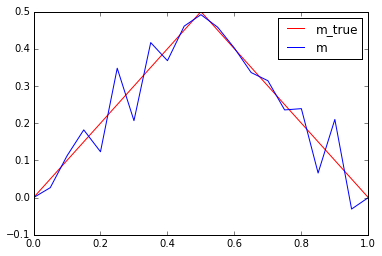
$\mathbf{m} = \left( I + \Delta t\,K\right)^{n_t} \mathbf{d}.$

The code below shows that:

for a very coarse mesh (nx = 20) and no measurement noise (noise_std_dev = 0.0) the naive solution is quite good
for a finer mesh (nx = 100) and/or even small measurement noise (noise_std_dev = 1e-4) the naive solution is garbage

def naiveSolveInv(d):
    A = assembleMatrix(d.shape[0])
    
    p_i = d.copy()
    for i in np.arange(nt):
        p = A*p_i
        p_i[:] = p
        
    return p

T = 1.0
L = 1.0
k = 0.005

nx = 20
nt = 100

noise_std_dev = 1e-4

h = L/float(nx)
dt = T/float(nt)

x = np.linspace(0.+h, L-h, nx-1) #place nx-1 equispace point in the interior of [0,L] interval
#m_true = np.power(.5,-36)*np.power(x,20)*np.power(1. - x, 16)  #smooth true initial condition
m_true = 0.5 - np.abs(x-0.5)                                    #initial condition with a corner
u_true = solveFwd(m_true)

d = u_true + noise_std_dev*np.random.randn(u_true.shape[0])

m = naiveSolveInv(d)

plot(m_true, "-r", label = 'm_true')
plot(m, "-b", label = 'm')
plt.legend()
plt.show()

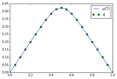
plot(u_true, "-b", label = 'u(T)')
plot(d, "og", label = 'd')
plt.legend()
plt.show()

png

Why does the naive solution fail?

Let $v_n = \sqrt{\frac{2}{L}} \sin\left( n \, \frac{\pi}{L} x \right)$ with $n=1,2,3, \ldots$, then we have that

$\mathcal{F} v_n = \lambda_n v_n, \quad \text{where the eigenvalues } \lambda_n = e^{-kT\left(\frac{\pi}{L} n \right)^2}.$

Note 1:

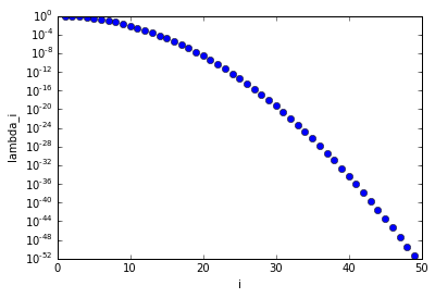
Large eigenvalues $\lambda_n$ corresponds to smooth eigenfunctions $v_n$;
Small eigenvalues $\lambda_n$ corresponds to oscillatory eigenfuctions $v_n$.

The figure below shows that the eigenvalues $\lambda_n$ decays extremely fast, that is the matrix $F$, discretization of the forward model $\mathcal{F}$, is extremely ill conditioned.

import numpy as np
import matplotlib.pyplot as plt
%matplotlib inline

T = 1.0
L = 1.0
k = 0.005

i = np.arange(1,50)
lambdas = np.exp(-k*T*np.power(np.pi/L*i,2))

plt.semilogy(i, lambdas, 'ob')
plt.xlabel('i')
plt.ylabel('lambda_i')
plt.show()

png

Note 2: The functions $v_n$, $n=1,2,3, \ldots$,form an orthonormal basis of $L^2([0,1])$.

That is, every function $f \in L^2([0,1])$ can be written as

$f = \sum_{n=1}^\infty \alpha_n v_n, \text{ where } \alpha_n = \int_0^1 f v_n dx.$

Consider now the noisy problem

$d = \mathcal{F}m_{\rm true} + \eta,$

where

$d$ is the data (noisy measurements)
$\eta$ is the noise: $\eta(x) = \sum_{n=1}^\infty \eta_n v_n(x)$
$m_{\rm true}$ is the true value of the parameter that generated the data
$\mathcal{F}$ is the forward heat equation

Then, the naive solution to the inverse problem $\mathcal{F}m = d$ is

$m = \mathcal{F}^{-1}d = \mathcal{F}^{-1}\left( \mathcal{F}m_{\rm true} + \eta \right) = m_{\rm true} + \mathcal{F}^{-1} \eta = m_{\rm true} + \mathcal{F}^{-1} \sum_{n=1}^{\infty} \eta_n v_n = m_{\rm true} + \sum_{n=1}^{\infty} \frac{\eta_n}{\lambda_n} v_n.$

If the coefficients $\eta_n = \int_0^1 \eta(x) \, v_n(x) \, dx$ do not decay sufficiently fast with respect to the eigenvalues $\lambda_n$, then the naive solution is unstable.

This implies that oscillatory components can not reliably be reconstructed from noisy data since they correspond to small eigenvalues.

Regularization by filtering

Remedy is to dampen the terms corresponding to small eigenvalues and write

$m \approx \sum_{n=1}^{\infty} \omega(\lambda_n^2)\, \lambda_n^{-1}\, \delta_n\, v_n,$

where

$\delta_n = \int_0^1 d(x) \, v_n(x) \, dx$ denotes the coefficients of the data $d$ in the basis $\left\{ v_n \right\}_{n=1}^\infty$ ;
$\omega( \lambda_n^2)$ is a filter function that allows to drop/stabilize the terms corresponding to small $\lambda_n$.

Truncated Singular Value Decomposition:

$\omega_\alpha( \lambda^2 ) = \left\{\begin{array}{ll} 1, & \text{ if } \lambda^2 \geq \alpha \\ 0, & \text{ otherwise}\end{array}, \right.$

where $\alpha$ is a regularization parameter.

Then, we have

$m_{\rm svd} = \sum_{n=1}^N \lambda_n^{-1} \delta_n\, v_n,$

where $N$ is largest index such that $\lambda_n^2 \geq \alpha$ (assuming that $\lambda_n$ are sorted in a decreasing order).

Tikhonov filter:

$\omega_\alpha( \lambda^2 ) = \frac{\lambda^2}{\lambda^2+\alpha},$ where $\alpha$ is a regularization parameter.

NOTE: $\omega_\alpha( \lambda^2 )$ is close to $1$ when $\lambda \gg \alpha$, close to 0 when $\lambda \ll \alpha$).

Then we have

$m_{\rm tikh} = \sum_{n=1}^{\infty} \frac{\lambda_n}{\lambda_n^2+\alpha} \delta_n\, v_n,$

def computeEigendecomposition(n):
    ## Compute F as a dense matrix
    F = np.zeros((n,n))
    m_i = np.zeros(n)
    
    for i in np.arange(n):
        m_i[i] = 1.0
        F[:,i] = solveFwd(m_i)
        m_i[i] = 0.0
    
    ## solve the eigenvalue problem
    lmbda, U = np.linalg.eigh(F)
    ## sort eigenpairs in decreasing order
    lmbda[:] = lmbda[::-1]
    lmbda[lmbda < 0.] = 0.0
    U[:] = U[:,::-1]
    
    return lmbda, U 


## Setup the problem
T = 1.0
L = 1.0
k = 0.005

nx = 100
nt = 100

noise_std_dev = 0.0#1e-3

h = L/float(nx)
dt = T/float(nt)

## Compute the data d by solving the forward model
x = np.linspace(0.+h, L-h, nx-1)
#m_true = np.power(.5,-36)*np.power(x,20)*np.power(1. - x, 16)
m_true = 0.5 - np.abs(x-0.5)
u_true = solveFwd(m_true)
d = u_true + noise_std_dev*np.random.randn(u_true.shape[0])

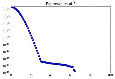
## Compute eigenvector and eigenvalues of the discretized forward operator
lmbda, U = computeEigendecomposition(nx-1)

plt.semilogy(lmbda, 'ob')
plt.title("Eigenvalues of F")
plt.show()

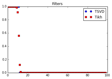
# Show filters
alpha = 1.e-6
plt.plot(lmbda*lmbda >= alpha, 'ob', label="TSVD")
plt.plot(lmbda*lmbda/(lmbda*lmbda + alpha), 'sr', label="Tikh")
plt.legend()
plt.title("Filters")
plt.show()

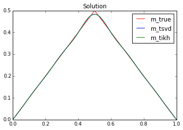
# Compute TSVD and Tikh sol
lmbda_inv = np.zeros_like(lmbda)
lmbda_inv[lmbda >= np.sqrt(alpha)] = lmbda[lmbda >= np.sqrt(alpha)]**(-1)
m_tsvd = np.dot(U, lmbda_inv*np.dot(U.T, d))

den = lmbda*lmbda+alpha
m_tikh = np.dot(U, (lmbda/den)*np.dot(U.T, d))

plot(m_true, "-r", label = 'm_true')
plot(m_tsvd, "-b", label = 'm_tsvd')
plot(m_tikh, "-g", label = 'm_tikh')
plt.title("Solution")
plt.legend()
plt.show()

png

This file is part of the hIPPYlib library. For more information and source code availability see https://hippylib.github.io.

hIPPYlib is free software; you can redistribute it and/or modify it under the terms of the GNU General Public License (as published by the Free Software Foundation) version 2.0 dated June 1991.

Computational and Variational Methods for Inverse Problems

Fall 2017, CSE 397/GEO 391/ME 397/ORI 397
Prof. O. Ghattas & Dr. U. Villa
Jupyter Notebooks

An illustrative example

1D Inverse Heat Equation

Forward problem

Analytical solution to the forward problem.

Inverse problem

Ill-posedness of the inverse problem

Discretization

Semidiscretization in space

Time discretization

A naive solution to the inverse problem

Why does the naive solution fail?

Regularization by filtering

Truncated Singular Value Decomposition:

Tikhonov filter:

Computational and Variational Methods for Inverse Problems

Fall 2017, CSE 397/GEO 391/ME 397/ORI 397Prof. O. Ghattas & Dr. U. VillaJupyter Notebooks

An illustrative example

1D Inverse Heat Equation

Forward problem

Analytical solution to the forward problem.

Inverse problem

Ill-posedness of the inverse problem

Discretization

Semidiscretization in space

Time discretization

A naive solution to the inverse problem

Why does the naive solution fail?

Regularization by filtering

Truncated Singular Value Decomposition:

Tikhonov filter:

Fall 2017, CSE 397/GEO 391/ME 397/ORI 397
Prof. O. Ghattas & Dr. U. Villa
Jupyter Notebooks