Coefficient field inversion in an elliptic partial differential equation

We consider the estimation of a coefficient in an elliptic partial differential equation as a first model problem. Depending on the interpretation of the unknowns and the type of measurements, this model problem arises, for instance, in electrical impedence tomography.

Let \(\Omega\subset\mathbb{R}^n\), \(n\in\{1,2,3\}\) be an open, bounded domain and consider the following problem:

\[\min_{m} J(m):=\frac{1}{2}\int_{\Omega} (u-d)^2\, dx + \frac{\gamma}{2}\int_\Omega|\nabla m|^2\,dx,\]

where \(u\) is the solution of

\[\begin{split} \quad -\nabla\cdot(e^m \nabla u) &= 0 \text{ in }\Omega,\\ e^m \nabla u &= j \text{ on }\partial\Omega. \end{split}\]

Here \(m \in \mathcal{M}:=\{m\in L^{\infty}(\Omega) \bigcap H^1(\Omega)\}\) denotes the unknown parameter field, \(u \in \mathcal{V}:= \left\{v \in H^1(\Omega): v(\boldsymbol{x}_c) = 0 \text{ for a given point } \boldsymbol{x}_c\in \Omega \right\}\) the state variable, \(d\) the (possibly noisy) data, \(j\in H^{-1/2}(\partial\Omega)\) a given boundary force, and \(\gamma\ge 0\) the regularization parameter.

The variational (or weak) form of the forward problem:

Find \(u\in \mathcal{V}\) such that

\[\int_{\Omega}e^m \nabla u \cdot \nabla \tilde{p} \, dx - \int_{\partial \Omega} j \tilde{p} \,dx = 0, \text{ for all } \tilde{p}\in \mathcal{V}.\]

Gradient evaluation:

The Lagrangian functional \(\mathscr{L}:\mathcal{V}\times\mathcal{M}\times\mathcal{V}\rightarrow \mathbb{R}\) is given by

\[\mathscr{L}(u,m,p):= \frac{1}{2}\int_{\Omega}(u-u_d)^2 dx + \frac{\gamma}{2}\int_\Omega \nabla m \cdot \nabla m dx + \int_{\Omega} e^m\nabla u \cdot \nabla p dx - \int_{\partial \Omega} j\,p\, dx.\]

Then the gradient of the cost functional \(\mathcal{J}(m)\) with respect to the parameter \(m\) in an arbitrary direction \(\tilde m\) is

\[(\mathcal{G}(m), \tilde m) := \mathscr{L}_m(u,m,p)(\tilde{m}) = \gamma \int_\Omega \nabla m \cdot \nabla \tilde{m}\, dx + \int_\Omega \tilde{m}e^m\nabla u \cdot \nabla p\, dx \quad \forall \tilde{m} \in \mathcal{M},\]

where \(u \in \mathcal{V}\) is the solution of the forward problem,

\[(\mathscr{L}_p(u,m,p), \tilde{p}) := \int_{\Omega}e^m\nabla u \cdot \nabla \tilde{p}\, dx - \int_{\partial\Omega} j\,\tilde{p}\, dx = 0 \quad \forall \tilde{p} \in \mathcal{V},\]

and \(p \in \mathcal{V}\) is the solution of the adjoint problem,

\[(\mathscr{L}_u(u,m,p), \tilde{u}) := \int_{\Omega} e^m\nabla p \cdot \nabla \tilde{u}\, dx + \int_{\Omega} (u-d)\tilde{u}\,dx = 0 \quad \forall \tilde{u} \in \mathcal{V}.\]

Steepest descent method.

Written in abstract form, the steepest descent methods computes an update direction \(\hat{m}_k\) in the direction of the negative gradient defined as

\[\int_\Omega \hat{m}_k \tilde{m}\, dx = -\left(\mathcal{G}(m_k), \tilde m\right) \quad \forall \tilde{m} \in \mathcal{M},\]

where the evaluation of the gradient \(\mathcal{G}(m_k)\) involve the solution \(u_k\) and \(p_k\) of the forward and adjoint problem (respectively) for \(m = m_k\).

Then we set \(m_{k+1} = m_k + \alpha \hat{m}_k\), where the step length \(\alpha\) is chosen to guarantee sufficient descent.

Goals:

By the end of this notebook, you should be able to:

solve the forward and adjoint Poisson equations
understand the inverse method framework
visualise and understand the results
modify the problem and code

Mathematical tools used:

Finite element method
Derivation of gradient via the adjoint method
Armijo line search

Import dependencies

import matplotlib.pyplot as plt
%matplotlib inline

import dolfin as dl
from hippylib import nb

import numpy as np
import logging


logging.getLogger('FFC').setLevel(logging.WARNING)
logging.getLogger('UFL').setLevel(logging.WARNING)
dl.set_log_active(False)

np.random.seed(seed=1)

Model set up:

As in the introduction, the first thing we need to do is to set up the numerical model.

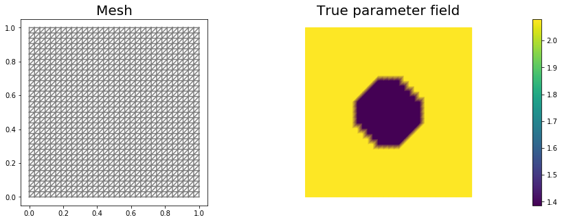
In this cell, we set the mesh mesh, the finite element spaces Vm and Vu corresponding to the parameter space and state/adjoint space, respectively. In particular, we use linear finite elements for the parameter space, and quadratic elements for the state/adjoint space.

The true parameter mtrue is the finite element interpolant of the function

\[m_{\rm true} = \left\{ \begin{array}{l} \ln 4 \; \forall \,(x,y) \, {\rm s.t.}\, \sqrt{ (x-.5)^2 + (y-.5)^2} \leq 0.2 \\ \ln 8 \; {\rm otherwise}. \end{array}\right.\]

The forcing term j for the forward problem is

\[j(x,y) = (x - 0.5)y(y-1) \; \forall {\boldsymbol{x}=(x,y)} \in \partial\Omega.\]

# create mesh and define function spaces
nx = 32
ny = 32
mesh = dl.UnitSquareMesh(nx, ny)
Vm = dl.FunctionSpace(mesh, 'Lagrange', 1)
Vu = dl.FunctionSpace(mesh, 'Lagrange', 2)

# The true and initial guess for inverted parameter
mtrue_str = 'std::log( 8. - 4.*(pow(x[0] - 0.5,2) + pow(x[1] - 0.5,2) < pow(0.2,2) ) )'
mtrue = dl.interpolate(dl.Expression(mtrue_str, degree=5), Vm)

# define function for state and adjoint
u = dl.Function(Vu)
m = dl.Function(Vm)
p = dl.Function(Vu)

# define Trial and Test Functions
u_trial, m_trial, p_trial = dl.TrialFunction(Vu), dl.TrialFunction(Vm), dl.TrialFunction(Vu)
u_test,  m_test,  p_test  = dl.TestFunction(Vu),  dl.TestFunction(Vm),  dl.TestFunction(Vu)

# initialize input functions
j  = dl.Expression("(x[0]-.5)*x[1]*(x[1]-1)", degree=3)

# plot
plt.figure(figsize=(15,5))
nb.plot(mesh, subplot_loc=121, mytitle="Mesh", show_axis='on')
nb.plot(mtrue, subplot_loc=122, mytitle="True parameter field")
plt.show()

png

# Fix the value of the state at the center of the domain
def d_boundary(x,on_boundary):
    return dl.near(x[0], .5) and dl.near(x[1], .5)

u0 = dl.Constant(0.)
bc_state = dl.DirichletBC(Vu, u0, d_boundary, "pointwise")
bc_adj   = dl.DirichletBC(Vu, dl.Constant(0.), d_boundary, "pointwise")

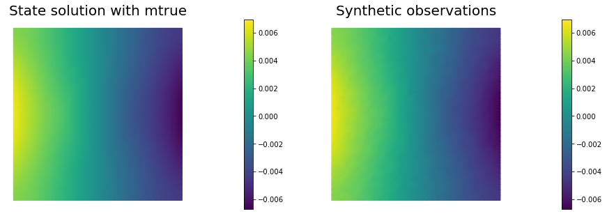
Set up synthetic observations (inverse crime):

To generate the synthetic observation we first solve the PDE for the state variable utrue corresponding to the true parameter mtrue. Specifically, we solve the variational problem

Find \(u\in \mathcal{V}\) such that

\(\underbrace{\int_\Omega e^{m_{\text true}} \nabla u \cdot \nabla v \, dx}_{\; := \; a_{\rm true}} - \underbrace{\int_{\partial\Omega} j\,v\,dx}_{\; := \;L_{\rm true}} = 0, \text{ for all } v\in \mathcal{V}\).

Then we perturb the true state variable and write the observation d as

\[d = u_{\rm true} + \eta, \quad {\rm where} \; \eta \sim \mathcal{N}(0, \sigma^2).\]

Here the standard variation \(\sigma\) is proportional to noise_level.

# noise level
noise_level = 0.01

# weak form for setting up the synthetic observations
a_true = dl.inner( dl.exp(mtrue) * dl.grad(u_trial), dl.grad(u_test)) * dl.dx
L_true = j * u_test * dl.ds

# solve the forward/state problem to generate synthetic observations
A_true, b_true = dl.assemble_system(a_true, L_true, bc_state)

utrue = dl.Function(Vu)
dl.solve(A_true, utrue.vector(), b_true)

d = dl.Function(Vu)
d.assign(utrue)

# perturb state solution and create synthetic measurements d
# d = u + ||u||/SNR * random.normal
MAX = d.vector().norm("linf")
noise = dl.Vector()
A_true.init_vector(noise,1)
noise.set_local( noise_level * MAX * np.random.normal(0, 1, len(d.vector().get_local())) )
bc_adj.apply(noise)

d.vector().axpy(1., noise)

# plot
nb.multi1_plot([utrue, d], ["State solution with mtrue", "Synthetic observations"])
plt.show()

png

The cost functional evaluation:

\[J(m):=\underbrace{\frac{1}{2}\int_\Omega (u-d)^2\, dx}_{\text misfit} + \underbrace{\frac{\gamma}{2}\int_\Omega|\nabla m|^2\,dx}_{\text reg}\]

# Regularization parameter
gamma = 1e-9

# Define cost function
def cost(u, d, m, gamma):
    reg = 0.5*gamma * dl.assemble( dl.inner(dl.grad(m), dl.grad(m))*dl.dx ) 
    misfit = 0.5 * dl.assemble( (u-d)**2*dl.dx)
    return [reg + misfit, misfit, reg]

Setting up the variational form for the state/adjoint equations and gradient evaluation

Below we define the variational forms that appears in the the state/adjoint equations and gradient evaluations.

Specifically,

a_state, L_state stand for the bilinear and linear form of the state equation, repectively;
a_adj, L_adj stand for the bilinear and linear form of the adjoint equation, repectively;
grad_misfit, grad_reg stand for the contributions to the gradient coming from the data misfit and the regularization, respectively.

We also build the mass matrix \(M\) that is used to discretize the \(L^2(\Omega)\) inner product.

# weak form for setting up the state equation
a_state = dl.inner( dl.exp(m) * dl.grad(u_trial), dl.grad(u_test)) * dl.dx
L_state = j * u_test * dl.ds

# weak form for setting up the adjoint equations
a_adj = dl.inner( dl.exp(m) * dl.grad(p_trial), dl.grad(p_test) ) * dl.dx
L_adj = - dl.inner(u - d, p_test) * dl.dx

# weak form for gradient
grad_misfit = dl.inner(dl.exp(m)*m_test*dl.grad(u), dl.grad(p)) * dl.dx
grad_reg    = dl.Constant(gamma)*dl.inner(dl.grad(m), dl.grad(m_test))*dl.dx

# Mass matrix in parameter space
Mvarf    = dl.inner(m_trial, m_test) * dl.dx
M = dl.assemble(Mvarf)

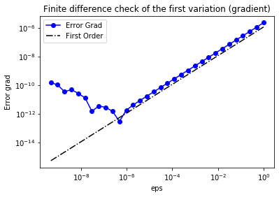
Finite difference check of the gradient

We use a finite difference check to verify that our gradient derivation is correct. Specifically, we consider a function \(m_0\in \mathcal{M}\) and we verify that for an arbitrary direction \(\tilde{m} \in \mathcal{M}\) we have

\[r := \left| \frac{ \mathcal{J}(m_0 + \varepsilon \tilde{m}) - \mathcal{J}(m_0)}{\varepsilon} - \left(\mathcal{G}(m_0), \tilde{m}\right)\right| = \mathcal{O}(\varepsilon).\]

In the figure below we show in a loglog scale the value of \(r\) as a function of \(\varepsilon\). We observe that \(r\) decays linearly for a wide range of values of \(\varepsilon\), however we notice an increase in the error for extremely small values of \(\varepsilon\) due to numerical stability and finite precision arithmetic.

m0 = dl.interpolate(dl.Constant(np.log(4.) ), Vm )

n_eps = 32
eps = np.power(2., -np.arange(n_eps))
err_grad = np.zeros(n_eps)

m.assign(m0)

#Solve the fwd problem and evaluate the cost functional
A, state_b = dl.assemble_system (a_state, L_state, bc_state)
dl.solve(A, u.vector(), state_b)

c0, _, _ = cost(u, d, m, gamma)

# Solve the adjoint problem and evaluate the gradient
adj_A, adjoint_RHS = dl.assemble_system(a_adj, L_adj, bc_adj)
dl.solve(adj_A, p.vector(), adjoint_RHS)

# evaluate the  gradient
grad0 = dl.assemble(grad_misfit + grad_reg)

# Define an arbitrary direction m_hat to perform the check 
mtilde = dl.Function(Vm).vector()
mtilde.set_local(np.random.randn(Vm.dim()))
mtilde.apply("")
mtilde_grad0 = grad0.inner(mtilde)

for i in range(n_eps):
    m.assign(m0)
    m.vector().axpy(eps[i], mtilde)
    
    A, state_b = dl.assemble_system (a_state, L_state, bc_state)
    dl.solve(A, u.vector(), state_b)

    cplus, _, _ = cost(u, d, m, gamma)
   
    err_grad[i] = abs( (cplus - c0)/eps[i] - mtilde_grad0 )

plt.figure()    
plt.loglog(eps, err_grad, "-ob", label="Error Grad")
plt.loglog(eps, (.5*err_grad[0]/eps[0])*eps, "-.k", label="First Order")
plt.title("Finite difference check of the first variation (gradient)")
plt.xlabel("eps")
plt.ylabel("Error grad")
plt.legend(loc = "upper left")
plt.show()

png

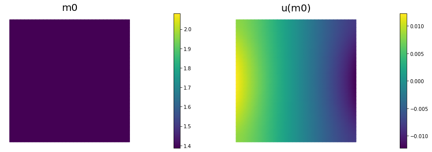
Initial guess

We solve the state equation and compute the cost functional for the initial guess of the parameter m0

m.assign(m0)

# solve state equation
A, state_b = dl.assemble_system (a_state, L_state, bc_state)
dl.solve(A, u.vector(), state_b)

# evaluate cost
[cost_old, misfit_old, reg_old] = cost(u, d, m, gamma)

# plot
plt.figure(figsize=(15,5))
nb.plot(m,subplot_loc=121, mytitle="m0", vmin=mtrue.vector().min(), vmax=mtrue.vector().max())
nb.plot(u,subplot_loc=122, mytitle="u(m0)")
plt.show()

png

The steepest descent with Armijo line search:

We solve the constrained optimization problem using the steepest descent method with Armijo line search.

The stopping criterion is based on a relative reduction of the norm of the gradient (i.e. \(\frac{\|g_{n}\|}{\|g_{0}\|} \leq \tau\)).

The gradient is computed by solving the state and adjoint equation for the current parameter \(m\), and then substituing the current state \(u\), parameter \(m\) and adjoint \(p\) variables in the weak form expression of the gradient:

\[(g, \tilde{m}) = \gamma(\nabla m, \nabla \tilde{m}) +(\tilde{m}e^m\nabla u, \nabla p).\]

The Armijo line search uses backtracking to find \(\alpha\) such that a sufficient reduction in the cost functional is achieved. Specifically, we use backtracking to find \(\alpha\) such that:

\[J( m - \alpha g ) \leq J(m) - \alpha c_{\rm armijo} (g,g).\]

# define parameters for the optimization
tol = 1e-4
maxiter = 1000
print_any = 10
plot_any = 50
c_armijo = 1e-5

# initialize iter counters
iter = 0
converged = False

# initializations
g = dl.Vector()
M.init_vector(g,0)

m_prev = dl.Function(Vm)

print( "Nit  cost          misfit        reg         ||grad||       alpha  N backtrack" )

while iter <  maxiter and not converged:

    # solve the adoint problem
    adj_A, adjoint_RHS = dl.assemble_system(a_adj, L_adj, bc_adj)
    dl.solve(adj_A, p.vector(), adjoint_RHS)

    # evaluate the  gradient
    MG = dl.assemble(grad_misfit + grad_reg)
    dl.solve(M, g, MG)

    # calculate the norm of the gradient
    grad_norm2 = g.inner(MG)
    gradnorm = np.sqrt(grad_norm2)
    
    if iter == 0:
        gradnorm0 = gradnorm

    # linesearch
    it_backtrack = 0
    m_prev.assign(m)
    alpha = 1.e5
    backtrack_converged = False
    for it_backtrack in range(20):
        
        m.vector().axpy(-alpha, g )

        # solve the forward problem
        state_A, state_b = dl.assemble_system(a_state, L_state, bc_state)
        dl.solve(state_A, u.vector(), state_b)

        # evaluate cost
        [cost_new, misfit_new, reg_new] = cost(u, d, m, gamma)

        # check if Armijo conditions are satisfied
        if cost_new < cost_old - alpha * c_armijo * grad_norm2:
            cost_old = cost_new
            backtrack_converged = True
            break
        else:
            alpha *= 0.5
            m.assign(m_prev)  # reset m
            
    if backtrack_converged == False:
        print( "Backtracking failed. A sufficient descent direction was not found" )
        converged = False
        break

    sp = ""
    if (iter % print_any)== 0 :
        print( "%3d %1s %8.5e %1s %8.5e %1s %8.5e %1s %8.5e %1s %8.5e %1s %3d" % \
            (iter, sp, cost_new, sp, misfit_new, sp, reg_new, sp, \
            gradnorm, sp, alpha, sp, it_backtrack) )

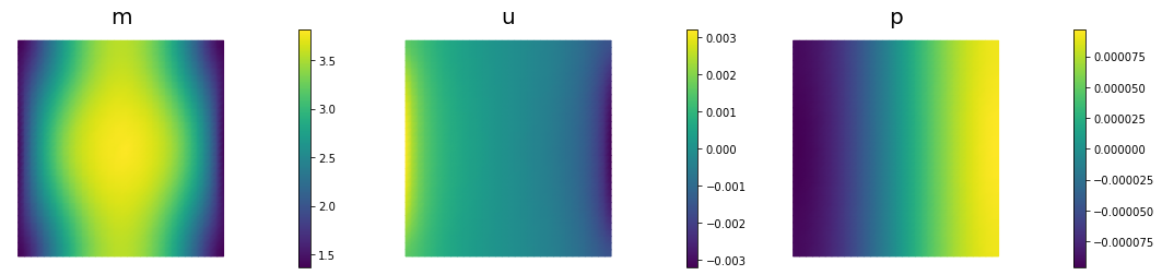
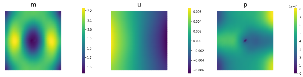
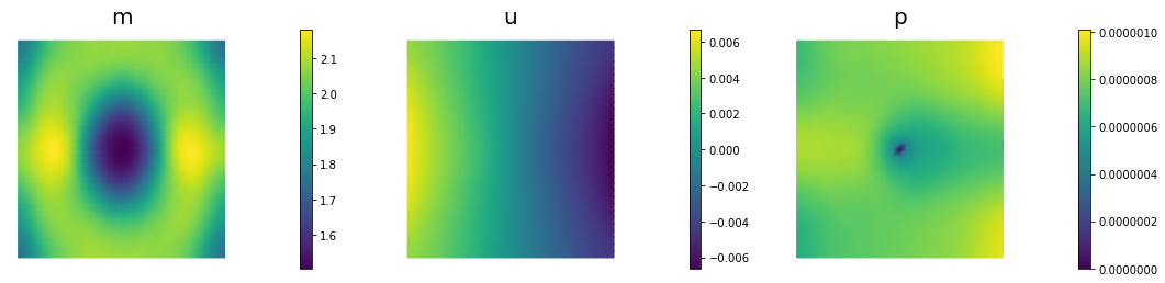
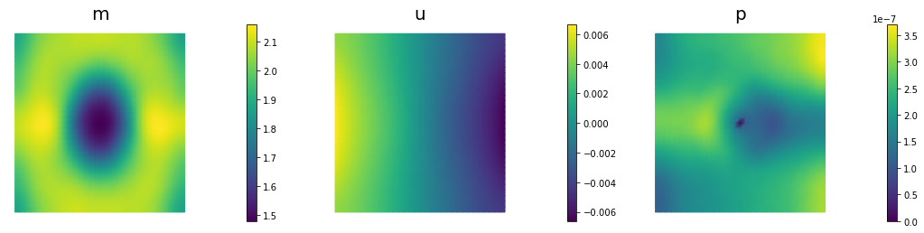
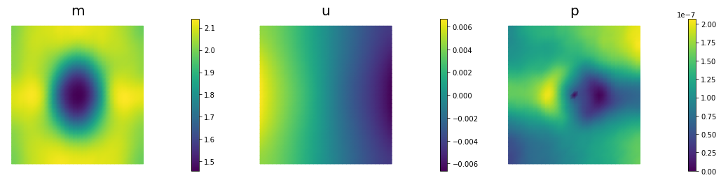
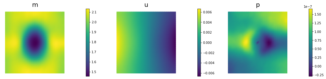
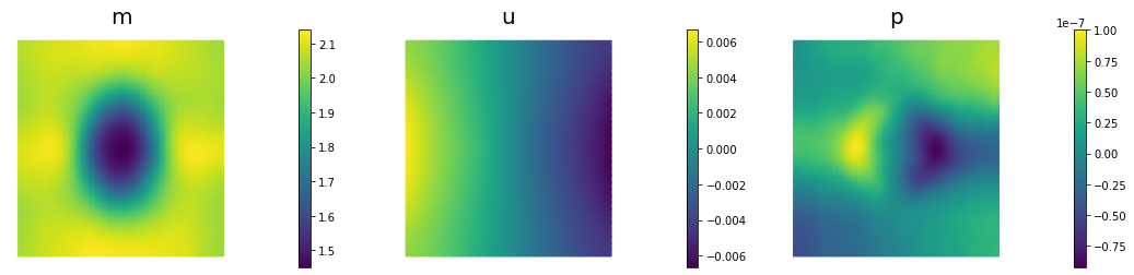
    if (iter % plot_any)== 0 :
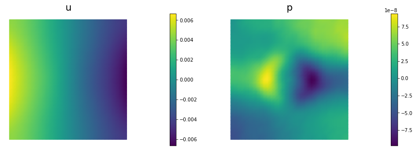
        nb.multi1_plot([m,u,p], ["m","u","p"], same_colorbar=False)
        plt.show()
    
    # check for convergence
    if gradnorm < tol*gradnorm0 and iter > 0:
        converged = True
        print ("Steepest descent converged in ",iter,"  iterations")
        
    iter += 1
    
if not converged:
    print ( "Steepest descent did not converge in ", maxiter, " iterations")

Nit  cost          misfit        reg         ||grad||       alpha  N backtrack
  0   2.98997e-06   2.97418e-06   1.57877e-08   1.72104e-05   1.00000e+05     0

png

 3.51785e-08   2.73244e-08   7.85413e-09   4.88854e-07   1.00000e+05     0
 9.29867e-09   7.76578e-09   1.53288e-09   3.85679e-07   2.50000e+04     2
 6.29728e-09   4.77456e-09   1.52271e-09   1.14065e-07   5.00000e+04     1
 5.04096e-09   3.59688e-09   1.44408e-09   9.00238e-08   2.50000e+04     2
 4.47367e-09   3.11925e-09   1.35442e-09   3.97325e-08   1.00000e+05     0

png

 4.02951e-09   2.75056e-09   1.27895e-09   9.32922e-08   2.50000e+04     2
 3.76667e-09   2.54619e-09   1.22048e-09   6.30495e-08   2.50000e+04     2
 3.55225e-09   2.38594e-09   1.16631e-09   3.03959e-08   5.00000e+04     1
 3.36957e-09   2.24964e-09   1.11993e-09   2.82392e-08   5.00000e+04     1
 3.23058e-09   2.14439e-09   1.08618e-09   4.07865e-08   2.50000e+04     2

png

 3.13196e-09   2.07166e-09   1.06030e-09   2.94700e-08   2.50000e+04     2
 3.05004e-09   2.01557e-09   1.03447e-09   1.65672e-08   1.00000e+05     0
 2.97722e-09   1.95997e-09   1.01725e-09   2.07193e-08   5.00000e+04     1
 2.91441e-09   1.91212e-09   1.00230e-09   3.11788e-08   2.50000e+04     2
 2.86792e-09   1.87840e-09   9.89526e-10   1.48662e-08   5.00000e+04     1

png

 2.82690e-09   1.84718e-09   9.79719e-10   2.11316e-08   2.50000e+04     2
 2.79441e-09   1.82313e-09   9.71283e-10   1.09647e-08   5.00000e+04     1
 2.76686e-09   1.80197e-09   9.64885e-10   1.45394e-08   2.50000e+04     2
 2.74511e-09   1.78625e-09   9.58861e-10   8.34227e-09   1.00000e+05     0
 2.72362e-09   1.76882e-09   9.54806e-10   2.16296e-08   2.50000e+04     2

png

 2.70897e-09   1.75721e-09   9.51760e-10   1.50883e-08   2.50000e+04     2
 2.69585e-09   1.74685e-09   9.49000e-10   7.45019e-09   5.00000e+04     1
 2.68434e-09   1.73733e-09   9.47013e-10   1.02607e-08   2.50000e+04     2
 2.67489e-09   1.72954e-09   9.45344e-10   5.61049e-09   5.00000e+04     1
 2.66740e-09   1.72332e-09   9.44084e-10   7.15164e-09   5.00000e+04     1

png

 2.66009e-09   1.71683e-09   9.43252e-10   1.08026e-08   2.50000e+04     2
 2.65455e-09   1.71197e-09   9.42577e-10   5.14606e-09   5.00000e+04     1
 2.64955e-09   1.70737e-09   9.42189e-10   7.30712e-09   2.50000e+04     2
 2.64550e-09   1.70360e-09   9.41897e-10   3.83880e-09   5.00000e+04     1
 2.64233e-09   1.70059e-09   9.41738e-10   5.05905e-09   5.00000e+04     1

png

 2.63906e-09   1.69732e-09   9.41740e-10   7.81137e-09   2.50000e+04     2
 2.63667e-09   1.69490e-09   9.41772e-10   3.60998e-09   5.00000e+04     1
 2.63445e-09   1.69254e-09   9.41904e-10   5.27256e-09   2.50000e+04     2
 2.63279e-09   1.69074e-09   9.42049e-10   3.80767e-09   2.50000e+04     2
 2.63131e-09   1.68908e-09   9.42226e-10   2.18974e-09   1.00000e+05     0

png

 2.62982e-09   1.68736e-09   9.42460e-10   5.72602e-09   2.50000e+04     2
 2.62879e-09   1.68611e-09   9.42674e-10   4.01567e-09   2.50000e+04     2
 2.62785e-09   1.68495e-09   9.42906e-10   1.99582e-09   5.00000e+04     1
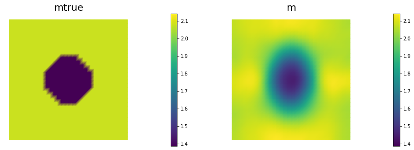
Steepest descent converged in  382   iterations

nb.multi1_plot([mtrue, m], ["mtrue", "m"])
nb.multi1_plot([u,p], ["u","p"], same_colorbar=False)
plt.show()

png

This file is part of cmis_labs, the teaching material for ESE 5932 Computational Methods for Imaging Science at Washington University in St. Louis. Please see https://uvilla.github.io/cmis_labs for more information and source code availability.

We would like to acknowledge the Extreme Science and Engineering Discovery Environment (XSEDE), which is supported by National Science Foundation grant number ACI-1548562, for providing cloud computing resources (Jetstream) for this course through allocation TG-SEE190001.