Poisson Equation in 2D

In this example we solve the Poisson equation in two space dimensions.

For a domain $\Omega \subset \mathbb{R}^2$ with boundary $\partial \Omega = \Gamma_D \cup \Gamma_N$, we write the boundary value problem (BVP):

\[\left\{ \begin{array}{ll} - \Delta u = f & \text{in} \; \Omega, \\ u = u_D & \text{on} \; \Gamma_D, \\ \nabla u \cdot \boldsymbol{n} = g & \text{on} \; \Gamma_N. \end{array} \right.\]

Here, $\Gamma_D \subset \Omega$ denotes the part of the boundary where we prescribe Dirichlet boundary conditions, and $\Gamma_N \subset \Omega$ denotes the part of the boundary where we prescribe Neumann boundary conditions. $\boldsymbol{n}$ denotes the unit normal of $\partial \Omega$ pointing outside $\Omega$.

To obtain the weak form we define the functional spaces $V_{u_D} := \left\{ u \in H^1(\Omega) \, |\, u = u_D \text{ on } \Gamma_D \right\}$ and $V_{0} := \left\{ u \in H^1(\Omega) \, |\, u = 0 \text{ on } \Gamma_D \right\}$. Then we multiply the strong form by an arbitrary function $v \in V_0$ and integrate over $\Omega$:

\[- \int_\Omega \Delta u \, v \, dx = \int_\Omega f\,v \, dx, \quad \forall v \in V_0.\]

Integration by parts of the non-conforming term gives

\[- \int_\Omega \Delta u \, v \, dx = \int_\Omega \nabla u \cdot \nabla v \, dx - \int_{\partial\Omega} (\nabla u \cdot \boldsymbol{n}) \,v\, ds\]

Recalling that $v = 0$ on $\Gamma_D$ and that $\nabla u \cdot \boldsymbol{n} = g$ on $\Gamma_N$, the weak form of the BVP is the following.

Find $u \in V_{u_D}$:

\[\int_\Omega \nabla u \cdot \nabla v \, dx = \int_\Omega f\,v \, dx + \int_{\Gamma_N} g\,v\,ds, \quad \forall v \in V_0.\]

To obtain the finite element discretization we then introduce a triangulation (mesh) $\mathcal{T}_h$ of the domain $\Omega$ and we define a finite dimensional subspace $V_h \subset H^1(\Omega)$ consisting of globally continuous functions that are piecewise polynomial on each element of $\mathcal{T}_h$.

By letting $V_{h, u_D} := \{ v_h \in V_h: \, v_h = u_D \text{ on } \Gamma_D\}$ and $V_{h, 0} := \{ v_h \in V_h: v_h = 0 \text{ on } \Gamma_D\}$, the finite element method then reads:

Find $u_h \in V_{h, u_D}$ such that:

\[\int_\Omega \nabla u_h \cdot \nabla v_h \, dx = \int_\Omega f\,v_h \, dx + \int_{\Gamma_N} g\,v_h\,ds, \quad \forall v_h \in V_{h,0}.\]

In what follow, we will let $\Omega := [0,1]\times[0,1]$ be the unit square, $\Gamma_N := \{ (x,y) \in \partial\Omega: \, y = 1\}$ be the top boundary, and $\Gamma_D := \partial\Omega \setminus \Gamma_N$ be the union of the left, bottom, and right boundaries.

The coefficient $f$, $g$, $u_D$ are chosen such that the analytical solution is $u_{ex} = e^{\pi y} \sin(\pi x)$.

1. Imports

We import the following Python packages:

dolfin is the python interface to FEniCS.
matplotlib is a plotting library that produces figure similar to the Matlab ones.
math is the python built-in library of mathematical functions.

# Import FEniCS
import dolfin as dl
import math

# Enable plotting inside the notebook
import matplotlib.pyplot as plt
%matplotlib inline

from hippylib import nb

import logging
logging.getLogger('FFC').setLevel(logging.WARNING)
logging.getLogger('UFL').setLevel(logging.WARNING)
dl.set_log_active(False)

2. Define the mesh and the finite element space

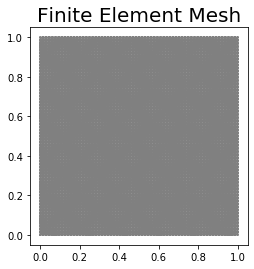
We define a triangulation (mesh) of the unit square $\Omega = [0,1]\times[0,1]$ with n elements in each direction. The mesh size $h$ is $\frac{1}{n}$.

We also define the finite element space $V_h$ as the space of globally continuos functions that are piecewise polinomial (of degree $d$) on the elements of the mesh.

n = 64
d = 1
mesh = dl.UnitSquareMesh(n, n)
Vh = dl.FunctionSpace(mesh, "Lagrange", d)
print("Number of dofs", Vh.dim())
nb.plot(mesh, mytitle="Finite Element Mesh", show_axis='on')
plt.show()

Number of dofs 4225

png

3. Define the Dirichlet boundary condition

We define the Dirichlet boundary condition $u = u_d := \sin(\pi x)$ on $\Gamma_D$.

def boundary_d(x, on_boundary):
    return (x[1] < dl.DOLFIN_EPS or x[0] < dl.DOLFIN_EPS or x[0] > 1.0 - dl.DOLFIN_EPS) and on_boundary

u_d  = dl.Expression("sin(DOLFIN_PI*x[0])", degree = d+2)
bcs = [dl.DirichletBC(Vh, u_d, boundary_d)]

4. Define the variational problem

We write the variational problem $a(u_h, v_h) = F(v_h)$. Here, the bilinear form $a$ and the linear form $L$ are defined as

\[a(u_h, v_h) := \int_\Omega \nabla u_h \cdot \nabla v_h \, dx\]
$L(v_h) := \int_\Omega f v_h \, dx + \int_{\Gamma_N} g \, v_h \, dx$.

$u_h$ denotes the trial function and $v_h$ denotes the test function. The coefficients $f = 0$ and $g = \pi\, e^{\pi y} \sin( \pi x)$ are also given.

uh = dl.TrialFunction(Vh)
vh = dl.TestFunction(Vh)

f = dl.Constant(0.)
g = dl.Expression("DOLFIN_PI*exp(DOLFIN_PI*x[1])*sin(DOLFIN_PI*x[0])", degree=d+2)
a = dl.inner(dl.grad(uh), dl.grad(vh))*dl.dx
L = f*vh*dl.dx + g*vh*dl.ds

5. Assemble and solve the finite element discrete problem

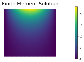
We now assemble the finite element stiffness matrix $A$ and the right hand side vector $b$. Dirichlet boundary conditions are applied at the end of the finite element assembly procedure and before solving the resulting linear system of equations.

A, b = dl.assemble_system(a, L, bcs)
uh = dl.Function(Vh)
dl.solve(A, uh.vector(), b)

nb.plot(uh, mytitle="Finite Element Solution")
plt.show()

png

6. Compute error norms

We then compute the $L^2(\Omega)$ and the energy norm of the difference between the exact solution and the finite element approximation.

u_ex = dl.Expression("exp(DOLFIN_PI*x[1])*sin(DOLFIN_PI*x[0])", degree = d+2, domain=mesh)
grad_u_ex = dl.Expression( ("DOLFIN_PI*exp(DOLFIN_PI*x[1])*cos(DOLFIN_PI*x[0])",
                         "DOLFIN_PI*exp(DOLFIN_PI*x[1])*sin(DOLFIN_PI*x[0])"), degree = d+2, domain=mesh )

norm_u_ex   = math.sqrt(dl.assemble(u_ex**2*dl.dx))
norm_grad_ex = math.sqrt(dl.assemble(dl.inner(grad_u_ex, grad_u_ex)*dl.dx))

err_L2   = math.sqrt(dl.assemble((uh - u_ex)**2*dl.dx))
err_grad = math.sqrt(dl.assemble(dl.inner(dl.grad(uh) - grad_u_ex, dl.grad(uh) - grad_u_ex)*dl.dx))

print ("|| u_ex - u_h ||_L2 / || u_ex ||_L2 = ", err_L2/norm_u_ex)
print ("|| grad(u_ex - u_h)||_L2 / = || grad(u_ex)||_L2 ", err_grad/norm_grad_ex)

|| u_ex - u_h ||_L2 / || u_ex ||_L2 =  0.00042675397744578077
|| grad(u_ex - u_h)||_L2 / = || grad(u_ex)||_L2  0.02453704048509311

This file is part of cmis_labs, the teaching material for ESE 5932 Computational Methods for Imaging Science at Washington University in St. Louis. Please see https://uvilla.github.io/cmis_labs for more information and source code availability.

We would like to acknowledge the Extreme Science and Engineering Discovery Environment (XSEDE), which is supported by National Science Foundation grant number ACI-1548562, for providing cloud computing resources (Jetstream) for this course through allocation TG-SEE190001.