Image Denoising: Tikhonov regularization

Given a possibly noisy image $d(\boldsymbol{x}) \in L^2(\Omega)$ defined within a rectangular domain $\Omega \subset \mathbb{R}^2$, we would like to find the image $m(\boldsymbol{x}) \in H^1(\Omega)$ that is closest in the $L_2(\Omega)$ sense, i.e. we want to minimize

\[\mathcal{J}_{LS}(m) := \frac{1}{2}\int_\Omega (m - d)^2 \; d\boldsymbol{x},\]

while also removing noise, which is assumed to comprise very rough components of the image.

This latter goal can be incorporated as an additional term in the objective, in the form of a penalty, called regularization.

Here we consider a Tikhonov regularization functional of the form

\[\alpha \mathcal{R}_{TN}(m) := \! \frac{\alpha}{2}\int_\Omega \nabla m \cdot \! \nabla m \; d\boldsymbol{x},\]

where $\alpha$ acts as a diffusion coefficient that controls how strongly we impose the penalty, i.e. how much smoothing occurs.

Thus the denoised image $m \in H^1(\Omega)$ is the minimizer of the functional

\[\mathcal{J}(m) := \mathcal{J}_{LS}(m) + \alpha \mathcal{R}_{TN}(m).\]

First order necessary optimality conditions

Let $\delta_m \mathcal{J}(m, \tilde{m})$ denote the first variation of $\mathcal{J}(m)$ in the direction $\tilde{m}$, i.e.

\[\delta_m \mathcal{J}(m, \tilde{m}) := \lim_{\varepsilon \rightarrow 0} \frac{\mathcal{J}(m + \varepsilon \tilde{m}) - \mathcal{J}(m)}{\varepsilon} = \left. \frac{d}{d \varepsilon} \mathcal{J}(m + \varepsilon \tilde{m})\right|_{\varepsilon=0}.\]

The necessary condition is that the first variation of $\mathcal{J}(m)$ equals to $0$ for all directions $\tilde{m} \in H^1(\Omega)$:

\[\delta_m \mathcal{J} = 0 \Longleftrightarrow \frac{d}{d \varepsilon} \mathcal{J}(m + \varepsilon \tilde{m}) = 0 \quad \forall \tilde{m} \in H^1(\Omega).\]

Variational form:

To obtain the variational form of the necessary optimality conditions we follow the steps below.

1) Expand the one dimensional function $\phi(\varepsilon) := \mathcal{J}(m + \varepsilon \tilde{m})$ as

\[\mathcal{J}(m + \varepsilon \tilde{m}) = \frac{1}{2}\int_\Omega (m + \varepsilon \tilde{m} - d)^2 \; d\boldsymbol{x} + \frac{\alpha}{2}\int_\Omega \nabla (m +\varepsilon \tilde{m})\cdot \! \nabla (m +\varepsilon \tilde{m}) \; d\boldsymbol{x}.\]

2) Differentiate the one dimensional function $\phi(\varepsilon)$ with respect to $\varepsilon$

\[\frac{d \phi}{d \varepsilon} = \int_\Omega \tilde{m} (m + \varepsilon \tilde{m} - d) \; d\boldsymbol{x} + \alpha\int_\Omega \nabla \tilde{m} \cdot \! \nabla (m +\varepsilon \tilde{m}) \; d\boldsymbol{x}.\]

3) Evaluate $\frac{d \phi}{d \varepsilon}$ at $\varepsilon = 0$

\[\delta_m \mathcal{J}(m, \tilde{m}) = \left. \frac{d \phi}{d \varepsilon} \right|_{\varepsilon=0} = \int_\Omega \tilde{m} (m - d) \; d\boldsymbol{x} + \alpha\int_\Omega \nabla \tilde{m} \cdot \! \nabla m \; d\boldsymbol{x}.\]

4) Set $\delta_m \mathcal{J}(m, \tilde{m}) = 0$ for all $\tilde{m} \in H^1(\Omega)$. That is find $m \in H^1(\Omega)$ such that:

\[\int_\Omega \tilde{m} (m - d) \; d\boldsymbol{x} + \alpha\int_\Omega \nabla \tilde{m} \cdot \! \nabla m \; d\boldsymbol{x} = 0 \quad \forall \tilde{m} \in H^1(\Omega).\]

Strong form:

To obtain the strong form, we invoke Green’s first identity and write

\[\alpha\int_\Omega \nabla \tilde{m} \cdot \! \nabla m \; d\boldsymbol{x} = -\alpha\int_\Omega \tilde{m} \nabla \cdot (\nabla m) \; d\boldsymbol{x} + \int_{\partial\Omega} \tilde{m} (\nabla m \cdot \boldsymbol{n}) d\boldsymbol{x},\]

where $\boldsymbol{n}$ is the outward unit normal vector to $\partial\Omega$.

By linearity of the integral we have

\[\int_\Omega \tilde{m} (-\alpha \nabla \cdot (\nabla m) + m - d) \; d\boldsymbol{x} + \int_{\partial\Omega} \tilde{m} (\nabla m \cdot \boldsymbol{n}) d\boldsymbol{x} = 0 \quad \forall \tilde{m}.\]

Assuming that $d$ is smooth enough, by arbitrarity of $\tilde{m} \in H^1(\Omega)$, the strong form the first order optimality conditions reads

\[\left\{ \begin{array}{ll} - \nabla \cdot (\alpha \nabla m) + m = d, & {\rm in} \; \Omega;\\ (\alpha \nabla m) \cdot \boldsymbol{n} = 0, & {\rm on} \; \partial\Omega. \end{array} \right.\]

The expression above corresponds to a boundary value problem with homogeneous Neumann condition $\nabla m \cdot \boldsymbol{n}=0$ on the boundary of $\Omega$, which amounts to assuming that the image intensity does not change normal to the boundary of the image.

1. Python imports

We import the following libraries:

math, which contains several mathematical functions
matplotlib, numpy, scipy, three libraries that together allow similar functionalities to matlab
dolfin, which allows us to discretize and solve variational problems using the finite element method
hippylib, the extesible framework I created to solve inverse problems in Python

Finally, we import the logging library to silence most of the output produced by dolfin.

import math

import matplotlib.pyplot as plt
%matplotlib inline

import numpy as np
import scipy.io as sio

import dolfin as dl

import hippylib as hp
from hippylib import nb


import logging

logging.getLogger('FFC').setLevel(logging.WARNING)
logging.getLogger('UFL').setLevel(logging.WARNING)
dl.set_log_active(False)

2. Geometry, true image, and data.

Read the true image from file, store the pixel values in data.
The width of the image is Lx = 1 and height Ly is set such that the aspect ratio of the image is preserved.
Generate a triangulation (pixelation) mesh of the region of interest.
Define the finite element space V of piecewise linear function on the elements of mesh. This represent the space of discretized images.
Interpolate the true image in the discrete space V. Call this interpolation m_true.
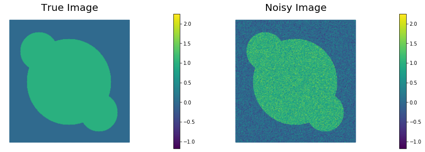
Corrupt the true image with i.i.d. Gaussian noise ($\sigma^2 = 0.09$) and interpolated the noisy image in the discrete space V. Call this interpolation d.
Visualize the true image m_true and the noisy image d.

data = sio.loadmat('circles.mat')['im']

Lx = 1.
h = Lx/float(data.shape[0])
Ly = float(data.shape[1])*h
  
mesh = dl.RectangleMesh(dl.Point(0,0),dl.Point(Lx,Ly),data.shape[0], data.shape[1])
V = dl.FunctionSpace(mesh, "Lagrange",1)

trueImage = hp.NumpyScalarExpression2D()
trueImage.setData(data, h, h)
m_true  = dl.interpolate(trueImage, V)

np.random.seed(seed=1)
noise_std_dev = .3
noise = noise_std_dev*np.random.randn(data.shape[0], data.shape[1])
noisyImage = hp.NumpyScalarExpression2D()
noisyImage.setData(data+noise, h, h)
d = dl.interpolate(noisyImage, V)

# Get min/max of noisy image, so that we can show all plots in the same scale
vmin = np.min(d.vector().get_local())
vmax = np.max(d.vector().get_local())

plt.figure(figsize=(15,5))
nb.plot(m_true, subplot_loc=121, mytitle="True Image", vmin=vmin, vmax = vmax)
nb.plot(d, subplot_loc=122, mytitle="Noisy Image", vmin=vmin, vmax = vmax)
plt.show()

png

3. Define misfit and regurization functionals and their variations.

Here we describe the variational forms for the $L_2$ misfit functional

\[\mathcal{J}_{LS}(m) := \frac{1}{2}\int_\Omega (m - d)^2 \; d\boldsymbol{x},\]

and the Tikhonov regularization functional

\[\mathcal{R}_{TN}(m) := \! \frac{1}{2}\int_\Omega \nabla m \cdot \! \nabla m \; d\boldsymbol{x}\]

By letting $\alpha > 0$ be the amount of regularization, the Tikhonov regularized functional $\mathcal{J}$ reads

\[\mathcal{J}(m) = \mathcal{J}_{LS}(m) + \alpha \mathcal{R}_{TN}(m) = \frac{1}{2}\int_\Omega (m - d)^2 \; d\boldsymbol{x} + \frac{\alpha}{2}\int_\Omega \nabla m \cdot \nabla m d\boldsymbol{x}.\]

The first variation of $\mathcal{J}$ is given by

\[\delta_m \mathcal{J}(m, \tilde{m}) = \int_\Omega \tilde{m} (m - d) \; d\boldsymbol{x} + \alpha\int_\Omega \nabla \tilde{m} \cdot \! \nabla m \; d\boldsymbol{x}.\]

Since we also know the true image m_true (this will not be the case for real applications), we can also compute the true $L_2$ error functional (mean square error MSE)L

\[{\rm MSE}(m) := \frac{1}{2}\int_\Omega (m - m_{\rm true})^2 \; d\boldsymbol{x}.\]

In the code below:

m = dl.Function(V) indicates the reconstructed image
m_tilde = dl.TestFunction(V) is a place holder for the arbitrary direction $\tilde{m}$
The function dl.solve(grad==0, m) solves the (possibly nonlinear) system of equations to set the first variation of $\mathcal{J}$ to $0$.
The function dl.assemble(form) evaluates the variational form form.

def TNsolution(alpha):
    m = dl.Function(V)
    m_tilde = dl.TestFunction(V)
    
    J_ls = dl.Constant(.5)*dl.inner(m - d, m - d)*dl.dx
    R_tn = dl.Constant(.5)*dl.inner(dl.grad(m), dl.grad(m))*dl.dx
    J = J_ls + dl.Constant(alpha)*R_tn
    
    grad = dl.inner(m - d, m_tilde)*dl.dx + dl.Constant(alpha)*dl.inner(dl.grad(m), dl.grad(m_tilde))*dl.dx
     
    dl.solve(grad==0, m)
    
    MSE = dl.inner(m - m_true, m - m_true)*dl.dx
    
    print( "{0:15e} {1:15e} {2:15e} {3:15e} {4:15e}".format(
           alpha, dl.assemble(J), dl.assemble(J_ls), dl.assemble(R_tn), dl.assemble(MSE)) )
    
    return m

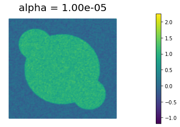
4. Reconstruction for different values of $\alpha$.

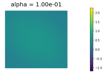
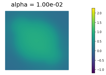
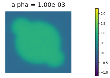
We define some values of $\alpha$ ($\alpha = 10^{-1}, 10^{-2}, 10^{-3}, 10^{-4}, 10^{-5}$) for the choice of the regularization paramenter.

Using the MSE as measure of image quality, the best reconstruction of the original image is obtained for $\alpha = 10^{-4}$. However, we could also use Morzov discrepancy principle or the L-curve to find a good choice of $\alpha$.

By looking at the reconstructed image, we notice that the sharp edges of the true image are a bit blurred in the reconstruction. This is one of the main shortcoming of Tikhonov regularization: more advanced types of regularization (like total variation regularization) should be used to better preserve edges in the reconstructed solution.

n_alphas = 5
alphas = np.power(10., -np.arange(1, n_alphas+1))

print( "{0:15} {1:15} {2:15} {3:15} {4:15}".format("alpha", "J", "J_ls", "R_tn", "MSE") )
for alpha in alphas:
    m = TNsolution(alpha)
    plt.figure()
    nb.plot(m, vmin=vmin, vmax = vmax, mytitle="alpha = {0:1.2e}".format(alpha))
    
plt.show()

alpha           J               J_ls            R_tn            MSE            
000000e-01    1.292136e-01    1.156620e-01    1.355154e-01    1.864769e-01
000000e-02    8.101481e-02    5.787655e-02    2.313825e+00    7.109993e-02
000000e-03    4.212558e-02    3.172326e-02    1.040233e+01    1.977690e-02
000000e-04    2.675885e-02    2.240033e-02    4.358520e+01    6.247110e-03
000000e-05    1.742607e-02    1.307915e-02    4.346922e+02    7.483126e-03

png

This file is part of cmis_labs, the teaching material for ESE 5932 Computational Methods for Imaging Science at Washington University in St. Louis. Please see https://uvilla.github.io/cmis_labs for more information and source code availability.

We would like to acknowledge the Extreme Science and Engineering Discovery Environment (XSEDE), which is supported by National Science Foundation grant number ACI-1548562, for providing cloud computing resources (Jetstream) for this course through allocation TG-SEE190001.